RL Post-Training: PPO and GRPO Variants #

Supervised fine-tuning (Section 1.5) teaches a model to imitate a fixed corpus, but imitation has intrinsic ceilings: the model can only reproduce behavior it was shown, and its objective rewards matching reference tokens rather than the outcome we actually care about, i.e., whether the response succeeds at the task at hand. This is a property of what the response does – something that two token sequences can satisfy equally well even when they share few tokens (and which a token-matching loss cannot see). Reinforcement learning (RL) post-training closes this gap. Instead of matching references, the model generates its own responses, each response is scored by a reward, and the model is updated to make high-reward responses more likely. This section develops that formulation generically — the objective, the policy-gradient estimator, and the two algorithms, PPO and GRPO, that dominate modern LLM post-training. Section 3 then applies this machinery to kernel generation, where the reward comes from compiling and running the generated code.

RL is especially effective when the reward is verifiable, i.e., it can be computed by an objective, automatic checker rather than a learned model of human preference. Math (check the final answer) and code (run unit tests) are the canonical cases, and this regime is known as RL with verifiable rewards (RLVR); kernel generation (compile, check against a reference, and profile) is another, and is the subject of Section 3.2.

The RL objective #

We model the post-trained LLM as a policy \( \pi_\theta(y \mid x) \) with parameters \( \theta \) that, given a prompt \( x \) , generates a response \( y \) autoregressively. Each response is scored by a scalar reward \( r(x, y) \in \mathbb{R} \) returned by an external verifier. Given a distribution of prompts \( \mathcal{D} \) , the RL objective is to maximize the expected reward of the responses the policy generates:

It is worth pointing out the sequential structure this compact objective hides. Generating a response is a sequence of decisions: at each step the policy observes a state, defined as the prompt plus the tokens emitted so far, \( (x, y_{\lt t}) \) , and subsequently then takes an action, the next token \( y_t \) . This autoregressive process continues until the response is completely generated. A full generation \( y \) is thus a trajectory, and \( \pi_\theta \) is a policy over trajectories. In the settings we care about, the reward is typically terminal and sparse, i.e., \( r(x, y) \) can be obtained only once the entire response has been produced (and, for verifiable domains, checked); so that there are no intermediate per-token rewards. This creates the central credit-assignment problem: a whole response earns a single scalar, yet that scalar gives no direct indication of which of the hundreds of token-level actions deserve the credit or blame. A slow kernel, for instance, might be 390 good tokens undone by one bad block-size choice, or wrong throughout; the reward is the same number in both cases. Separating the decisions that mattered from those that were incidental is precisely what the advantage estimators below are designed to do, though they operate at different granularities: PPO’s value network produces a per-position advantage, whereas GRPO’s group-relative baseline scores a whole response against its siblings, leaving credit within a response uniform. Sharpening credit below the response level (for instance by decomposing the reward across token classes such as reasoning vs. code) is a further step, taken up in Section 3.3.

To keep the policy from drifting too far from a reference model \( \pi_{\text{ref}} \) (typically the SFT model) — which stabilizes training and preserves the fluent, general behavior the model started with, a KL penalty is often added:

The essential contrast with SFT (Section 1.5): SFT minimizes a divergence to a fixed dataset, whereas RL maximizes reward over the policy’s own samples. This is what allows RL to reinforce a good response the model discovered on its own (even one that appears in no reference corpus) and thereby surpass the behavior imitation alone could reach.

Policy-gradient optimization #

Why policy gradients. Because the reward is a black box (we generally cannot backpropagate through a checker, a compiler, or a test harness), \( J(\theta) \) is optimized with policy-gradient methods, which estimate gradients from sampled rollouts alone.

Deriving the estimator. Deriving the gradient is worth a moment, because it explains why RL training takes the form it does. The difficulty is that \( \theta \) parameterizes the very distribution we average over, not just the quantity inside the average, so we cannot naively push the gradient through the expectation. Fixing a prompt \( x \) and writing the expectation as a sum over possible responses,

The right-hand side is not an expectation under \( \pi_\theta \) (the \( \nabla_\theta \pi_\theta \) factor is not a probability distribution), and \( r \) may be a non-differentiable black box, so we cannot estimate it by sampling as written. The log-derivative identity repairs this:

which is simply \( \nabla_\theta \log \pi_\theta = \nabla_\theta \pi_\theta / \pi_\theta \) rearranged. Substituting it restores a \( \pi_\theta(y \mid x) \) factor out front, turning the sum back into an expectation:

Restoring the average over prompts \( x \sim \mathcal{D} \) gives the policy-gradient theorem:

The REINFORCE rule. The payoff is that the gradient is once again an expectation over the policy’s own samples, so it can be estimated by Monte Carlo: draw responses from the current policy and average \( r(x,y)\, \nabla_\theta \log \pi_\theta(y \mid x) \) over them. The reward enters only as a scalar multiplier (it is never differentiated), and \( \nabla_\theta \log \pi_\theta \) is ordinary backpropagation through the model’s own log-probabilities, so a black-box, non-differentiable reward is no obstacle. This estimator is the classic REINFORCE rule.

What one Monte Carlo sample is. Concretely, one sample is one complete rollout: the policy generates a full response \( y = (y_1, \dots, y_T) \) token by token, and the oracle then returns a single terminal reward \( r(x, y) \) for the finished response (there is no reward for a half-written one). A single rollout already gives an unbiased gradient estimate, but its variance is high, so in practice one draws a batch of \( N \) independent rollouts per prompt and averages:

Each rollout contributes exactly one reward and one backprop pass; the per-token structure within a rollout (below) is deterministic bookkeeping, not additional sampling. Sampling several rollouts per prompt is also what makes the group-relative baseline of GRPO (discussed later) possible, since a single sample has nothing to compare against.

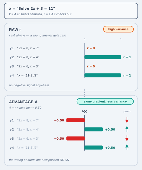
Four responses sampled for one prompt under a binary reward: subtracting the baseline \( b(x) = 0.50 \) — the typical reward for \( x \) — recenters \( r \in \{0, 1\} \) into an advantage of \( \pm 0.50 \) , which leaves the gradient unchanged in expectation while cutting its variance.

Reducing variance with a baseline. Intuitively, the update increases the log-probability of high-reward responses and decreases it for low-reward ones. The raw estimator is unbiased but high-variance, so in practice the reward is replaced by an advantage \( A(x,y) = r(x,y) - b(x) \) : a response-independent baseline \( b(x) \) (the typical reward for prompt \( x \) ) is subtracted to cut variance. This leaves the gradient unchanged in expectation, because the score function has zero mean and the log-derivative trick yields \( \mathbb{E}_{y \sim \pi_\theta}[\nabla_\theta \log \pi_\theta(y \mid x)] = \sum_y \nabla_\theta \pi_\theta(y \mid x) = \nabla_\theta \sum_y \pi_\theta(y \mid x) = \nabla_\theta 1 = 0 \) , so subtracting any such \( b(x) \) contributes nothing on average:

Spreading the reward over tokens. Since the response is a token sequence, the score term decomposes over tokens (the same autoregressive factorization as in SFT), which is how the sequence-level reward is distributed across per-token updates:

The choice of baseline/advantage estimator is what distinguishes the algorithms below.

PPO: Proximal Policy Optimization #

A learned baseline (actor-critic). Proximal Policy Optimization (PPO) [1] is the classic actor-critic instantiation. Alongside the policy (the “actor”), it trains a separate value network \( V_\phi(x, y_{\lt t}) \) (the “critic”) that predicts the reward a partial generation will eventually earn. This learned value serves as the baseline, so the advantage \( \hat{A}_t \) measures how much a continuation did better than the critic expected, position by position (in practice estimated with generalized advantage estimation, GAE). The hat denotes an estimate: the true advantage uses the unknown expected return, whereas \( \hat{A}_t \) is computed from \( V_\phi \) and a sampled rollout, so a well-trained critic gives a sharp, per-token signal while a poor one misleads the update.

Reusing rollouts via a probability ratio. Rollouts are expensive (for kernels, each one compiles and runs code), so PPO reuses a batch for several gradient steps rather than resampling after every step. Doing so correctly requires distinguishing the frozen sampling policy \( \pi_{\theta_{\text{old}}} \) that produced the batch from the current policy \( \pi_\theta \) being updated, and reweighting each sample by the probability ratio \( \rho_t(\theta) = \pi_\theta(y_t \mid x, y_{\lt t}) / \pi_{\theta_{\text{old}}}(y_t \mid x, y_{\lt t}) \) (importance sampling).

This is worth emphasizing: PPO does not merely change the baseline inside the vanilla policy gradient, it changes the loss function itself. Plain REINFORCE optimizes a surrogate that contains only the current policy,

which is valid only for samples drawn from the very \( \pi_\theta \) being differentiated, so it must be resampled after a single step. PPO replaces the \( \log \pi_\theta \) term with the ratio \( \rho_t(\theta) \) , which references a second, frozen policy and is exactly what lets a batch sampled from \( \pi_{\theta_{\text{old}}} \) be reused for multiple updates. (The learned value baseline of the previous paragraph is a baseline choice allowed within the vanilla framework; the ratio, and the clipping below, genuinely change the objective.)

Clipping (the “proximal” part). Importance reweighting is only trustworthy while \( \pi_\theta \) stays close to \( \pi_{\theta_{\text{old}}} \) ; if \( \rho_t \) grows large, a few samples dominate and the update can blow up. PPO therefore clips the ratio, optimizing the minimum of the unclipped and clipped terms:

The \( \min \) makes the clipping one-sided in exactly the right way, which is clearest by cases on the sign of the advantage:

• Positive advantage ( \( \hat{A}_t \gt 0 \) , a good token). We want to raise this token’s probability, so \( \rho_t \) tends to grow. Once \( \rho_t \gt 1+\epsilon \) , the clipped term \( (1+\epsilon)\hat{A}_t \) is smaller than the unclipped \( \rho_t \hat{A}_t \) , so the \( \min \) selects it and the objective goes flat: no further reward for pushing the probability even higher.
• Negative advantage ( \( \hat{A}_t \lt 0 \) , a bad token). We want to lower its probability, so \( \rho_t \) tends to shrink. Once \( \rho_t \lt 1-\epsilon \) , the clipped term \( (1-\epsilon)\hat{A}_t \) (recall \( \hat{A}_t \lt 0 \) ) is again the one the \( \min \) selects, flattening the objective: no further reward for suppressing it beyond the band.

Either way, once a token’s ratio leaves \( [1-\epsilon, 1+\epsilon] \) (a typical \( \epsilon \) is 0.1 to 0.2) its gradient contribution vanishes, keeping each update inside a trust region around the sampling policy. At the first step, \( \theta = \theta_{\text{old}} \) so \( \rho_t = 1 \) and the gradient matches plain policy gradient; the ratio and clip only bite as \( \theta \) drifts. (This clipping of the probability ratio is distinct from clipping the reward itself, a separate stabilization device: some verifiable-reward systems bound the reward’s magnitude, e.g. capping a speedup reward, so that a single rare extreme value cannot dominate the update.)

The cost. PPO is robust and is the algorithm behind much of RLHF, but it is expensive: the value network is a second model roughly the size of the policy, so it roughly doubles memory and adds its own training instability (a bad critic yields misleading advantages). That overhead is the specific pain point the next algorithm removes.

GRPO: Group Relative Policy Optimization #

The group as its own baseline. Group Relative Policy Optimization (GRPO) [2] removes the value network entirely and has become the workhorse of modern LLM RL, including the kernel-generation systems of Section 3.2. Its motivating question is: the critic exists only to answer “what reward should I expect for this prompt?”, so can we estimate that reference point from samples instead of a trained model? GRPO does exactly that. For each prompt \( x \) it samples a group of \( G \) complete responses from the current policy,

scores each with the reward oracle to get \( r_i = r(x, y_i) \) , and uses the group’s mean reward as the baseline. The advantage of a response is how far its reward sits above or below that mean, normalized by the group’s spread:

Reading the advantage:

• \( \hat{A}_i \gt 0 \) : response \( i \) beat its siblings on this prompt, so reinforce it.
• \( \hat{A}_i \lt 0 \) : it was worse than its siblings, so suppress it.
• \( \hat{A}_i \approx 0 \) : it was about average, so little signal.

Every token of response \( y_i \) is assigned this same sequence-level \( \hat{A}_i \) , since there is no critic to produce a per-token value. This uniform assignment can be relaxed without reintroducing a critic: one can partition a response into token classes and run a separate group-relative objective on each, giving the classes different advantages. TritonRL [5] does exactly this for kernels, crediting the reasoning (plan) tokens and the code tokens with distinct rewards; we return to it in Section 3.3. The group’s rollouts thus do double duty: they are both the samples the gradient is averaged over and the samples whose mean provides the baseline, which is precisely what lets GRPO drop the value network. Everything else is inherited from PPO: GRPO plugs this \( \hat{A}_i \) into the same clipped-ratio surrogate (with the same \( \rho \) and the same trust-region logic).

Per prompt, not per batch. A group is tied to a single prompt: the mean and standard deviation are computed within each prompt’s group, never pooled across prompts. A training batch is a collection of such groups, one per prompt. This within-group normalization is what makes the baseline fair: a response is judged against other attempts at the same prompt, so an easy prompt (rewards near 1.0) and a hard one (rewards near 0.1) each reward their own best attempts, rather than the update simply favoring whichever prompt happened to be easier. It also means GRPO structurally requires \( G \gt 1 \) : with a single response there is no group, no mean to subtract, and the advantage is undefined (contrast PPO, whose critic-based baseline works even for one rollout per prompt).

The zero-variance pitfall. The group baseline is informative only when the rewards actually differ. If every response in a group earns the same reward, then \( r_i = \operatorname{mean} \) for all \( i \) , so every \( \hat{A}_i = 0 \) and the prompt contributes no gradient at all. This happens when a group is all-fail (nothing compiles, common early in training) or all-pass (a prompt the model already solves). GRPO therefore learns only from prompts in a learnable band that still produce a mix of outcomes, which is exactly why curriculum and dynamic task selection matter for it (Section 3.2).

Normalization. The division by \( \operatorname{std}(\{r_1, \dots, r_G\}) \) rescales advantages to unit variance per prompt. It is a normalization choice, not a necessity: dropping it (together with the sequence-length normalization) removes a subtle bias toward longer or harder responses (Dr. GRPO [3]). The essential idea, the group mean as baseline, does not depend on it: the kernel-generation system TritonRL [5], for example, uses the mean-only advantage \( \hat{A}_i = r_i - \operatorname{mean}(\{r_1, \dots, r_G\}) \) with no division by the standard deviation.

KL regularization to the reference policy #

Both algorithms are often combined with the KL term from the objective above, penalizing divergence from the reference policy \( \pi_{\text{ref}} \) (typically the SFT model). Concretely, for GRPO the full training loss adds a KL penalty (weighted by \( \beta \) ) to the clipped surrogate:

The ratio \( \rho_{i,t} \) is PPO’s probability ratio, now indexed by response \( i \) and token \( t \) (PPO uses the identical loss with its critic-based \( \hat{A}_t \) in place of \( \hat{A}_i \) ). The KL term’s role is to keep the policy within a trust region in distribution space: it stabilizes optimization and prevents the model from drifting away from the fluent, general behavior it started with as it chases reward. Note this is a second, distinct closeness constraint from the clipping: clipping keeps \( \pi_\theta \) near the sampling policy \( \pi_{\theta_{\text{old}}} \) (an optimization safeguard for reusing a batch), whereas the KL term keeps it near the fixed reference \( \pi_{\text{ref}} \) (preserving general capability). Some large-scale RLVR recipes deliberately weaken or drop the KL term when they want the policy to move far from the reference, relying on other mechanisms for stability (DAPO [4]).

References #

RL algorithms.

1. J. Schulman, F. Wolski, P. Dhariwal, A. Radford, and O. Klimov. Proximal Policy Optimization Algorithms. arXiv:1707.06347, 2017. arxiv.org/abs/1707.06347
2. Z. Shao, P. Wang, Q. Zhu, R. Xu, J. Song, X. Bi, et al. DeepSeekMath: Pushing the Limits of Mathematical Reasoning in Open Language Models (introduces GRPO). arXiv:2402.03300, 2024. arxiv.org/abs/2402.03300
3. Z. Liu, C. Chen, W. Li, P. Qi, T. Pang, C. Du, W. S. Lee, and M. Lin. Understanding R1-Zero-Like Training: A Critical Perspective (Dr. GRPO). arXiv:2503.20783, 2025. arxiv.org/abs/2503.20783
4. Q. Yu, Z. Zhang, R. Zhu, Y. Yuan, et al. DAPO: An Open-Source LLM Reinforcement Learning System at Scale. arXiv:2503.14476, 2025. arxiv.org/abs/2503.14476
5. J. Woo, S. Zhu, A. Nie, Z. Jia, Y. Wang, and Y. Park. TritonRL: Training LLMs to Think and Code Triton Without Cheating. arXiv:2510.17891, 2025. arxiv.org/abs/2510.17891