Supervised Fine-Tuning on Kernel Corpora #

Section 1 assembled the target of this tutorial. It laid out the accelerator hardware a kernel must run on (Section 1.1), showed how the compiler stack handles the common case while leaving a long tail of kernels to be written by hand (Section 1.2), and introduced the CUDA, Triton, and NKI languages those kernels are written in (Section 1.3) — closing on the point that the kernel is precisely the artifact we would now like an LLM to produce. This section takes up that problem: how to post-train a general-purpose model into a capable kernel generator.

The gap to close is real. A pretrained LLM has read an enormous amount of general text and code, but it has never been trained specifically to be a kernel-writing agent. Asked to produce a CUDA, Triton, or NKI kernel for a given operator, hardware target, and set of constraints, a base model will often return code that is syntactically invalid or poorly designed — mixing APIs, inventing nonexistent intrinsics, or emitting broken launch configurations.

Supervised fine-tuning (SFT) is the first and most direct remedy: we assemble a corpus of high-quality (task, kernel) examples and train the model to imitate them via next-token prediction. This does two things at once. It grounds the model in the basic syntax and APIs of the target kernels — often enough on its own to yield valid, idiomatic code — and it reshapes the model’s behavioral prior toward the right region of the output space. That prior is useful in itself, and it also gives later post-training (such as the reinforcement learning of Section 3.2) a much stronger starting point.

SFT Data Curation with Kernel Corpora #

Hand-written or agent-written kernels exist for the long tail of AI workloads, fused GEMM epilogues, FlashAttention-style online softmax, MoE routing, quantized/heterogeneous fusion. Using the existing kernel examples, the SFT data can be constructed as follows:

\[ \mathcal{D}_{SFT} = \big\{ (x^{(i)}, y^{(i)}) \big\}_{i=1}^{N}, \]

where each prompt $ x^{(i)} $ encodes everything the model is given as input, and each target $ y^{(i)} $ is the desired output. For kernel generation, a prompt $ x $ typically bundles together the operator specification (e.g., a reference PyTorch function), the hardware target and constraints (dtype, shapes, memory limits), and any instruction or few-shot framing; the target $ y $ is a reference kernel (e.g., a Triton program) that correctly and efficiently implements the operator.

For instance, TritonRL’s task instruction explicitly invites the model to fuse operators and explore algorithmic improvements (naming examples such as combining a matmul with a following activation, or using an online-softmax formulation) and pins the output format (real compilable code, a fixed module name, no pseudocode or test harness), which both biases generation toward the fused long-tail kernels we care about and keeps completions parseable for automatic verification. Both $ x $ and $ y $ are token sequences drawn from a shared vocabulary $ \mathcal{V} $ :

\[ x = (x_1, \dots, x_{|x|}), \qquad y = (y_1, \dots, y_{|y|}), \qquad x_j, y_t \in \mathcal{V}. \]

As a concrete example, consider a training pair $ (x, y) $ for a fused RMSNorm kernel. Root-mean-square normalization (RMSNorm) is a normalization layer used throughout modern transformers: it rescales each feature vector by its root-mean-square magnitude, then applies a learned per-feature gain. Concretely, for one input row $ a \in \mathbb{R}^{N} $ (the last dimension of the tensor) with a learnable weight $ w \in \mathbb{R}^{N} $ and a small constant $ \epsilon $ for numerical stability, the output $ b \in \mathbb{R}^{N} $ is

\[ \mathrm{RMS}(a) = \sqrt{\frac{1}{N}\sum_{j=1}^{N} a_j^{2} + \epsilon}, \qquad b_j = \frac{a_j}{\mathrm{RMS}(a)}\, w_j \quad (j = 1, \dots, N). \]

Unlike LayerNorm, RMSNorm does not subtract the mean — it only divides by the RMS, which is why the reference below computes a reciprocal square root of the mean of squares and never centers the data.

The fused qualifier refers to how this is executed on the accelerator. Written naively, the layer is a chain of separate operators — square, a reduction to form the mean, add $ \epsilon $ , reciprocal-square-root, and two element-wise multiplies — and, as Section 1.3 discussed, running each as its own kernel would stream the row out to HBM and back between every step. RMSNorm has very low arithmetic intensity (a handful of FLOPs per element), so it is firmly memory-bound and those round-trips dominate its cost. A fused kernel performs the entire computation in one launch, loading $ a $ into on-chip memory once, computing $ \mathrm{RMS}(a) $ and the rescaling there, and writing only $ b $ back — exactly the kind of long-tail fusion that motivates hand-written kernels.

The training pair below encodes this task. The prompt $ x $ specifies the operator, the reference semantics, and the hardware target; the target $ y $ is the reference kernel the model is trained to reproduce.

Prompt $ x $ :

Write a Triton kernel that computes fused RMSNorm over the last dimension.
Input:  x of shape (M, N), fp16, on NVIDIA H100
Output: y of shape (M, N), fp16
Reference (PyTorch):
    def rmsnorm(x, w, eps=1e-6):
        rms = x.pow(2).mean(dim=-1, keepdim=True).add(eps).rsqrt()
        return x * rms * w

Target $ y $ :

import triton
import triton.language as tl

@triton.jit
def rmsnorm_kernel(x_ptr, w_ptr, y_ptr, N, eps,
                   BLOCK_N: tl.constexpr):
    row = tl.program_id(0)
    cols = tl.arange(0, BLOCK_N)
    mask = cols < N

    x = tl.load(x_ptr + row * N + cols, mask=mask, other=0.0).to(tl.float32)
    rms = tl.rsqrt(tl.sum(x * x, axis=0) / N + eps)
    w = tl.load(w_ptr + cols, mask=mask, other=0.0).to(tl.float32)

    y = (x * rms) * w
    tl.store(y_ptr + row * N + cols, y.to(tl.float16), mask=mask)

A brief description of the ground-truth Triton kernel: The fusion is the structure of the code. The whole square → reduce → reciprocal-square-root → rescale → gain chain lives in a single @triton.jit function, so it launches once. The row is pulled from HBM by exactly one tl.load at the top and the result written by exactly one tl.store at the bottom; in between, every intermediate, x * x, the reduced sum, rms, the gain w, the product y, is a value the compiler keeps in on-chip registers and passes straight to the next operation, never spilling it to HBM and reading it back.

That “written once, consumed immediately” shape is what lets the intermediates stay in registers, and it has a name in compiler terms: SSA (static single assignment), the intermediate form Triton and LLVM lower through (recall the Triton IR → LLVM IR → PTX → SASS path of Section 1.3). SSA’s one rule is that every value is assigned exactly once; a chain that reuses a name, such as

t = a * a        →   t1 = a * a
t = t / N        →   t2 = t1 / N
t = t + eps      →   t3 = t2 + eps

is rewritten into distinct versioned values t1, t2, t3. Because each value is defined once and its uses are explicit, the compiler can see that t1, t2, t3 are produced and consumed entirely within the kernel and never need a memory address — so they are allocated to registers rather than materialized in HBM. (The Python-level names x, rms, y you write are just ordinary variables; SSA is what they become after lowering.) A separate but complementary detail visible in the code is the .to(tl.float32) / .to(tl.float16) pair: the reduction is accumulated in fp32 for numerical accuracy and only the final result is cast back to the fp16 output dtype — and keeping that fp32 working copy costs nothing precisely because it already lives in registers.

An unfused implementation would instead be several kernels — square, mean, rsqrt, multiply — each reloading its input from HBM and writing its output back. For a chain of $ k $ such ops over a row of $ n $ bytes that is roughly $ 2kn $ bytes of HBM traffic, versus about $ 2n $ for the fused kernel (one read, one write) — the $ k $ -fold reduction from Section 1.3. Keeping the reduction and the rescale on-chip is what makes this memory-bound operator efficient, and it is the concrete payoff the prompt $x$ was asking for when it said fused. The one simplification here is that the kernel assumes a full row fits in one tile ( $ \texttt{BLOCK\_N} \ge N $ , one program per row); a kernel for very large $ N $ would tile the reduction across blocks and combine partial sums, but the fusion principle is unchanged.

The corpus $ \mathcal{D}_{SFT} $ is simply a collection of many such pairs spanning different operators, shapes, dtypes, and hardware targets.

Sampling #

SFT targets are drawn from two broad sources: expert examples (human-written or library/vendor kernels) and teacher models (a strong model prompted to synthesize kernels for each task). In both cases the raw samples are noisy, so the practical question is how to sample and select the pairs that go into the corpus.

It is worth being precise about what “sampling” means for each source, because the word carries two related senses. There is no single canonical kernel for a task — many different Triton programs correctly and efficiently implement the same operator, differing in tiling, block sizes, and scheduling. For a teacher model, sampling is meant in its literal statistical sense: as Section 3.2 will make precise, an autoregressive model defines a probability distribution $ \pi_{\text{teacher}}(y \mid x) $ over kernels $ y $ given a task prompt $ x $ , and to sample is to draw a concrete kernel from that distribution by generating tokens with randomness (a nonzero decoding temperature) rather than always taking the single highest-probability (greedy) continuation. Because the draw is stochastic, prompting the teacher on the same task twice yields two different kernels — which is precisely what lets us collect many distinct candidates per task. For expert examples, “sampling” is meant in the looser sense of selecting which existing kernels to pull into the corpus.

Either way the raw draws are noisy: a stochastic teacher produces some kernels that do not compile or are subtly wrong, and mined corpora contain low-value or duplicated code. So the practical work has two parts — sampling (drawing candidates so they are diverse and plentiful) and selection (filtering the draws down to trustworthy training targets). Several complementary techniques address these:

Parallel sampling (for diversity). For each task, draw $ K $ candidate kernels from the teacher via stochastic decoding rather than a single greedy decode, and keep all valid candidates rather than selecting one. Because there is no single canonical kernel for a task, different samples explore different tiling and scheduling strategies, so retaining several implementations per task broadens the corpus and prevents the model from collapsing onto a single style. This is why systems like TritonRL sample many candidate kernels per task (up to ten in their case), each paired with its own reasoning trace, rather than keeping a single generation. Concretely, TritonRL draws its tasks from KernelBook (a dataset of PyTorch reference implementations, not to be confused with the KernelBench evaluation benchmark), takes roughly 11.6K executable references, wraps each in an instruction to produce a Triton kernel, and prompts a frontier teacher model for up to ten completions per task; the surviving pairs distill that teacher’s expertise into a much smaller 8B student. The teacher is itself a design choice: distilling the same task set from two different teachers (DeepSeek-R1 and GPT-OSS-120B) yields two distinct students of roughly 60K examples each.

To make this concrete, the same fused RMSNorm task from above admits several valid but distinct kernels. Below are Triton sketches of three; they compute identical RMSNorm but differ in how the row is tiled and reduced.

(A) One row per program — the kernel from earlier: the whole row fits in one tile, reduced in a single pass. row = tl.program_id(0) assigns one program to each row, and cols = tl.arange(0, BLOCK_N) (with BLOCK_N >= N) covers the entire row in a single tile, so the whole reduction is the one tl.sum(x * x, axis=0); the row is read from HBM exactly once by the single tl.load and the result written by the single tl.store.

@triton.jit
def rmsnorm_A(x_ptr, w_ptr, y_ptr, N, eps, BLOCK_N: tl.constexpr):
    row  = tl.program_id(0)              # one program per row
    cols = tl.arange(0, BLOCK_N)         # BLOCK_N >= N: whole row in one tile
    mask = cols < N
    x   = tl.load(x_ptr + row * N + cols, mask=mask, other=0.0).to(tl.float32)
    rms = tl.rsqrt(tl.sum(x * x, axis=0) / N + eps)   # single-pass reduce
    w   = tl.load(w_ptr + cols, mask=mask, other=0.0).to(tl.float32)
    tl.store(y_ptr + row * N + cols, (x * rms * w).to(tl.float16), mask=mask)

(B) Blocked reduction — for a row too large to hold on-chip: loop over column chunks to accumulate the sum of squares, then loop again to normalize. The first for off in range(0, N, BLOCK_N) loop walks the row in BLOCK_N-wide chunks, and acc += tl.sum(x * x, axis=0) accumulates the running sum of squares across them before rms = tl.rsqrt(acc / N + eps) finalizes it; the second loop then re-loads each chunk and applies the normalization in the tl.store. Note that the row is therefore read from HBM twice — once per loop — which is the cost of not being able to hold it on-chip.

@triton.jit
def rmsnorm_B(x_ptr, w_ptr, y_ptr, N, eps, BLOCK_N: tl.constexpr):
    row = tl.program_id(0)
    acc = 0.0                                          # pass 1: sum of squares
    for off in range(0, N, BLOCK_N):
        cols = off + tl.arange(0, BLOCK_N)
        mask = cols < N
        x    = tl.load(x_ptr + row * N + cols, mask=mask, other=0.0).to(tl.float32)
        acc += tl.sum(x * x, axis=0)
    rms = tl.rsqrt(acc / N + eps)
    for off in range(0, N, BLOCK_N):                   # pass 2: normalize + write
        cols = off + tl.arange(0, BLOCK_N)
        mask = cols < N
        x    = tl.load(x_ptr + row * N + cols, mask=mask, other=0.0).to(tl.float32)
        w    = tl.load(w_ptr + cols, mask=mask, other=0.0).to(tl.float32)
        tl.store(y_ptr + row * N + cols, (x * rms * w).to(tl.float16), mask=mask)

(C) Multi-row block — one program handles BLOCK_M rows at once via a 2-D tile, reducing along the feature axis. rows = pid * BLOCK_M + tl.arange(0, BLOCK_M) selects a block of rows and offs = rows[:, None] * N + cols[None, :] builds a 2-D (BLOCK_M, BLOCK_N) tile of offsets, so the single tl.load brings in several rows at once; tl.sum(x * x, axis=1) reduces along the feature axis to give one RMS value per row (a (BLOCK_M,) vector), and rms[:, None] / w[None, :] broadcast that per-row scale and the shared gain back across the tile in one fused multiply.

@triton.jit
def rmsnorm_C(x_ptr, w_ptr, y_ptr, M, N, eps,
              BLOCK_M: tl.constexpr, BLOCK_N: tl.constexpr):
    pid  = tl.program_id(0)
    rows = pid * BLOCK_M + tl.arange(0, BLOCK_M)       # a block of rows
    cols = tl.arange(0, BLOCK_N)                        # BLOCK_N >= N
    m2d  = (rows[:, None] < M) & (cols[None, :] < N)
    offs = rows[:, None] * N + cols[None, :]           # 2-D tile of offsets
    x    = tl.load(x_ptr + offs, mask=m2d, other=0.0).to(tl.float32)
    rms  = tl.rsqrt(tl.sum(x * x, axis=1) / N + eps)   # per-row reduce -> (BLOCK_M,)
    w    = tl.load(w_ptr + cols, mask=cols < N, other=0.0).to(tl.float32)
    y    = x * rms[:, None] * w[None, :]               # broadcast over rows
    tl.store(y_ptr + offs, y.to(tl.float16), mask=m2d)

The differences are summarized below:

Variant	Program → data	Reduction	Grid size	Best when	Main trade-off
A one-row	one program per row	one `tl.sum` over the full row (single tile)	$ M $	the row fits on-chip ( $ \texttt{BLOCK\_N} \ge N $ )	simplest; a single HBM read, but fails once $ N $ is too large
B blocked	one program per row	loop over column chunks, accumulate	$ M $	$ N $ too large for one tile	handles any $ N $ , but re-reads the row (two passes over HBM)
C multi-row	one program per $ \texttt{BLOCK\_M} $ rows	`tl.sum(..., axis=1)` on a 2-D tile	$ \lceil M / \texttt{BLOCK\_M} \rceil $	$ N $ small, many rows	better occupancy and load amortization; more registers per program

Rejection sampling (for quality). Pass the candidates through automatic verifiers and discard those that fail, keeping only kernels that clear three successive bars. Each stage catches a distinct failure a stochastic teacher will produce; taking the RMSNorm task as the running example:
1. Compiles. The candidate must build at all. Suppose a teacher forgets to mark BLOCK_N: tl.constexpr. Then BLOCK_N becomes an ordinary runtime argument (like N or eps), a value not known until the kernel is called. But tl.arange(0, BLOCK_N) uses that argument as the length of a tile, and in Triton a tile’s length is part of its tensor type: the compiler must know it at compile time to specialize the kernel. A runtime-valued length is therefore an error that Triton raises before generating any code, and the candidate is rejected immediately. (This is exactly why BLOCK_N is constexpr while N is not: N is only ever used as a value — in cols < N and the address arithmetic — whereas BLOCK_N sets a shape.)
2. Correct against the reference within numerical tolerance. This is where subtly-wrong kernels are caught — code that compiles and looks plausible but computes the wrong thing. Two classic cases: a kernel that subtracts the mean (computing LayerNorm rather than RMSNorm — recall RMSNorm never centers the data), or one that accumulates the sum of squares in fp16 instead of fp32 and drifts outside tolerance. Both pass stage 1 but fail here.
3. Clears a performance/speedup bar (optional). A kernel can be correct yet slow. One that leaves intermediates in HBM instead of fusing them on-chip, or picks a tiny BLOCK_N that starves occupancy, survives stages 1–2 but is cut here for missing the speedup threshold.
Filtering on these bars raises the quality floor of the corpus and is the main defense against training on subtly-wrong kernels (e.g., CUDA Agent filters candidates on correctness and speedup relative to reference implementations).
Source hygiene for expert examples. When mining existing corpora, prefer kernels that genuinely exercise the target programming model. Code that leaves the real computation to high-level framework ops teaches little about low-level kernel writing and is better filtered out or regenerated by a teacher. This takes two guises. The first is a mined target that is not a kernel at all — plain framework code such as return x * torch.rsqrt(x.pow(2).mean(-1, keepdim=True) + eps) * w, which belongs in the prompt as the reference but must never be used as the target y. The second, more insidious because it is kernel-shaped and slips past naive “does it use @triton.jit?” filters, keeps a real-looking @triton.jit function but does the actual work in the host wrapper that the test calls. Note that the torch op cannot go inside the kernel — a @triton.jit body is traced and lowered to Triton IR, and it operates on tile handles, not torch.Tensors, so a torch call there simply fails to compile. The cheat therefore lives one level up:
```
@triton.jit
def rmsnorm_kernel(x_ptr, y_ptr, N, BLOCK_N: tl.constexpr):
    # A sham kernel: it compiles and runs, but does NOT compute RMSNorm.
    # There is no sum-of-squares, no rsqrt, and no gain -- it just copies
    # the row through unchanged, so y == x.
    row  = tl.program_id(0)
    cols = tl.arange(0, BLOCK_N)
    mask = cols < N
    x = tl.load(x_ptr + row * N + cols, mask=mask)
    tl.store(y_ptr + row * N + cols, x, mask=mask)   # write input straight to output

def rmsnorm(x, w, eps=1e-6):        # host wrapper — this is what the test calls
    scratch = torch.empty_like(x)
    BLOCK_N = triton.next_power_of_2(x.shape[-1])    # arange length must be a power of two
    rmsnorm_kernel[(x.shape[0],)](x, scratch, x.shape[-1], BLOCK_N=BLOCK_N)
    # scratch now just holds a copy of x -- it is discarded, never returned:
    return torch.nn.functional.rms_norm(x, (x.shape[-1],), w, eps)  # real work, done by PyTorch
```
The wrapper does launch the kernel, so a check like “is a Triton kernel actually invoked?” passes — but its result (scratch) is discarded and the returned value comes entirely from the torch op. This passes a correctness check — the test calls rmsnorm, which returns the exact PyTorch result — yet the kernel demonstrates none of the tiling, on-chip reduction, or fusion the model is supposed to learn; the entire point has been handed back to the framework op the kernel was meant to replace. The same anti-pattern appears in RL settings as reward hacking (Section 2.3), where a model routes around a unit test with a torch call instead of writing a real kernel; in an SFT corpus it is just as corrosive, teaching the model that wrapping a framework call is an acceptable “kernel.” Such examples should be filtered out (or regenerated by a teacher) so the corpus rewards genuine low-level implementations. Catching the kernel-shaped variant takes more than a @triton.jit grep: TritonRL pairs a rule-based linter (which flags kernels that fall back on high-level framework ops) with an LLM judge that checks the code genuinely implements the operator. The stakes are concrete: kernel models fine-tuned on a signal that lacks such a functionality check have been observed to emit more functionally invalid kernels than their base model, because the unfiltered sham examples actively teach the shortcut.
Deduplication and difficulty balancing. Even after the filters above, the distribution of the surviving pairs matters, because the SFT loss is an average over examples — every extra copy of a pattern silently upweights it. Two skews are worth correcting.
- Deduplication. Parallel sampling and corpus mining both produce many near-identical kernels: a teacher drawn $ K $ times will often return the same implementation with only cosmetic differences (renamed variables, reordered lines, a different literal like BLOCK_N=512 vs. 1024, added comments), and scraped repos contain forks and copy-paste clones of popular kernels. Keeping all of them teaches the model that one pattern is far more probable than it should be. The fix is to deduplicate on normalized code — strip comments and whitespace and canonicalize identifiers, then compare by exact hash or by a near-duplicate similarity measure (e.g. token- or AST-level Jaccard/MinHash) — collapsing each cluster of clones to one representative. The distinction is what counts as “the same”: the A/B/C RMSNorm variants above are genuinely different algorithms and should all be kept, whereas two samples of variant A that differ only in block size or variable names are duplicates and should collapse to one.
- Difficulty balancing. Mined corpora are dominated by easy kernels — there are vastly more elementwise add/relu/copy examples than fused-attention or MoE-routing ones — and rejection sampling worsens the skew, because easy tasks yield far more surviving candidates than hard ones (a teacher lands a correct elementwise kernel almost every time, a fused long-tail kernel rarely). Left uncorrected, the model becomes fluent at trivial kernels and weak exactly on the long tail where hand-written kernels matter most (Section 1.3). The remedy is to label each task by difficulty — for instance the KernelBench tiers of single-operator (Level 1), operator-fusion (Level 2), and full-architecture (Level 3) kernels — and balance the corpus across those tiers and across operator categories, up-weighting the scarce hard cases (or ordering them into a curriculum) rather than letting the easy majority dominate the gradient. That said, harder is not always better: in TritonRL’s RL stage, training exclusively on single-operator (Level 1) tasks gave the best correctness and match-or-beat-reference rate on both single-operator and fusion (Level 2) evaluations, since fusion tasks succeed so rarely that they contribute little learnable signal while single-operator skill appears to transfer upward. The practical rule is to up-weight hard cases only while they still produce a usable training signal, not to over-index on tasks the model almost never solves.

The pairs that survive this sampling-and-selection process form the SFT corpus — a scalable source of execution-grounded supervision, which is often the only practical route to a corpus when few high-quality human-written kernels exist.

Data augmentation #

Sampling and selection give us a corpus of trustworthy (task, kernel) pairs, but each pair is still a bare input–output example: a task on one side, a kernel on the other. Before training, that raw supervision can be enriched — augmenting what each example teaches and how broadly the corpus covers the space — along three axes.

How one seed pair is multiplied into many. The seed is the single RMSNorm task and its kernel, and three augmentation axes fan out from it. One, reasoning: prepend a derivation — one program per row, reduce along the columns, memory-bound so fuse, BLOCK_N the next power of two, mask the tail, accumulate in fp32 — leaving the kernel unchanged, so the model reasons before it commits. Two, task and config: sweep across operators such as LayerNorm, softmax and RMSNorm-plus-residual, and within the operator sweep N, M, dtype and target, turning one pair into k pairs where the shape picks the variant. Three, metadata: tag the same pair with backend, difficulty and category, and put the tag in the prompt so generation can be conditioned and scarce backends up-weighted.

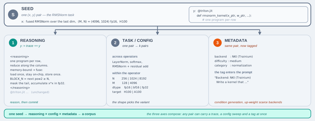
The three augmentation axes fanning out from one seed pair: prepending a reasoning trace, sweeping the task and its config into $ k $ pairs, and tagging the pair with metadata the prompt can condition on.

Reasoning augmentation. Instead of pairing a task only with its final kernel, each target is annotated with an explicit reasoning trace — a chain-of-thought that spells out the optimization decisions behind the code (tiling and block-size choices, memory-hierarchy staging such as shared-memory/SBUF interleaving, masking of boundary tiles, accumulation strategy, and so on). Such traces are typically distilled from a strong reasoning teacher: the teacher is prompted to both explain and implement the kernel, and the explanation is kept as part of the target $ y $ . Training on (task, reasoning + kernel) pairs teaches the model not merely to emit correct syntax, but to absorb the optimization knowledge itself, so that at inference time it reproduces the reasoning before committing to an implementation.

For the RMSNorm task from earlier, the augmented target $ y $ would prepend a trace like the following before the same kernel code:
```
<reasoning>
RMSNorm reduces over the last dim (N), so assign one program per row
(program_id(0)) and reduce along the columns.
The op is memory-bound, so fuse everything into one kernel: load the row
once, keep the sum-of-squares and rescale on-chip, write the row once.
Choose BLOCK_N as the next power of two >= N and mask cols < N for the tail.
Accumulate x*x in fp32 for numerical stability, then cast the result to fp16.
</reasoning>
@triton.jit
def rmsnorm_kernel(x_ptr, w_ptr, y_ptr, N, eps, BLOCK_N: tl.constexpr):
    ...   # the kernel shown earlier
```
The trace makes the why behind each line explicit — the one-program-per-row mapping, the fuse-to-stay-on-chip decision, the power-of-two BLOCK_N with masking, the fp32 accumulation — rather than leaving the model to reverse-engineer those choices from code alone.
Task augmentation. Coverage matters: a model exposed to a narrow set of tasks generalizes poorly to the long tail. The task pool is therefore diversified along two axes — across operators (different kernels and fusion patterns) and within an operator by varying its configuration, most importantly the input shapes and dtypes. Presenting the same operator under many shape/config regimes exposes the model to a broader range of performance scenarios (different memory-vs-compute trade-offs, tiling regimes, and occupancy constraints), which is essential for producing kernels that hold up across realistic workloads rather than a single benchmarked shape. These varied configurations can be generated automatically: TritonRL synthesizes extra input-generating functions with a teacher model, keeps up to five execution-validated shape variants per base task, and reports that this input augmentation improved one of its two distilled students by roughly 12% in correctness and 6% in the rate of matching or beating the reference on single-operator tasks, along with better robustness to unseen shapes.

Starting from the single RMSNorm task we have been using — (M, N) = (4096, 1024), fp16, on an H100 — augmentation expands it in both directions:
- Across operators: spin off related tasks — LayerNorm, fused RMSNorm + residual add, a SiLU/GELU activation, softmax — so the model sees a family of patterns rather than one.
- Within the operator: hold RMSNorm fixed but vary the configuration — N ∈ {256, 1024, 8192}, M ∈ {128, 4096}, dtype ∈ {fp16, bf16, fp32}, target ∈ {H100, A100}.
This second axis matters precisely because it changes the right implementation, connecting back to the A/B/C variants above: a small N favors the multi-row kernel (C), a large N that overflows on-chip memory forces the blocked reduction (B), and a mid-size N suits the one-row kernel (A). A corpus that contains RMSNorm only at N = 1024 would teach variant A and nothing else; varying the shape is what exposes the model to the full space of trade-offs.
Metadata augmentation. Beyond the task and kernel themselves, each example can be annotated with auxiliary information about the kernel — structured labels or tags describing properties the model cannot easily infer from the code alone (e.g., a difficulty label, the target hardware/backend, or the operator category). Such annotations can either condition generation (the label becomes part of the prompt $ x $ ) or organize training, for instance by balancing the corpus across categories or ordering examples into a curriculum.

The target-backend tag is a good example, and it matters because the same task maps to very different kernels across backends (Section 1.3): our RMSNorm task is a Triton program on an NVIDIA GPU but an NKI program on Trainium. Tagging each pair with its backend and surfacing that tag in the prompt,
```
Backend: NKI (AWS Trainium)      # <- metadata tag added to the prompt x
Write a kernel that computes fused RMSNorm over the last dimension.
...
```
lets one model serve every backend while generating the right dialect on demand, instead of silently blending CUDA, Triton, and NKI syntax. The same tag also organizes training: because backends are unevenly represented (abundant CUDA/Triton data, scarce NKI — the low-resource-DSL problem from Section 1.3), the corpus can be balanced or up-weighted by backend so the plentiful targets do not drown out the scarce ones.

Training on the kernel corpus #

With the corpus $ \mathcal{D}_{SFT} $ assembled and enriched, the training step is the standard SFT recipe of Section 1.5, now with kernels as the targets. We fine-tune an autoregressive policy $ \pi_\theta $ by maximum likelihood, minimizing the token-level negative log-likelihood of each reference kernel $ y^{(i)} $ given its task prompt $ x^{(i)} $ :

\[ \mathcal{L}_{\text{SFT}}(\theta) \;=\; -\,\frac{1}{N}\sum_{i=1}^{N} \sum_{t=1}^{|y^{(i)}|} \log \pi_\theta\!\big(y^{(i)}_t \mid x^{(i)}, \, y^{(i)}_{\lt t}\big). \]

As in Section 1.5, the loss is applied only to the kernel (completion) tokens under a loss mask, and it is teacher-forced: every position conditions on the ground-truth prefix rather than the model’s own past tokens. For kernels, the effect is exactly the two-fold grounding described at the start of this section, i.e., the model absorbs the target DSL’s syntax and API surface (the @triton.jit / nl.load idioms, valid launch configurations) and shifts its prior toward the region of well-formed, idiomatic kernels. The reasoning-augmented targets from above train it to reproduce the optimization reasoning before committing to code.

Limitations #

We have now seen SFT end to end: curate a corpus of (task, kernel) pairs, then train the model to maximize their likelihood token by token. It is a powerful and often indispensable first stage. But note that objective actually optimizes the probability of reproducing reference tokens, and it becomes clear that the very property that makes SFT simple and stable is also what bounds it. Three limitations follow directly, and together they set up why a second, reward-driven stage is needed.

Bounded by the demonstrations. SFT maximizes the likelihood of the reference kernels, so the trained model can at best reproduce the behavior it was shown — it has no mechanism to discover kernels better than those in its corpus. Its quality is capped by the strength of the teacher (or human experts) that produced the targets and by the curation filters; systematic mistakes or suboptimal schedules present in the data are absorbed faithfully rather than corrected.

Example: if every RMSNorm target in the corpus uses BLOCK_N = 1024, the model learns that block size even where 512 or 2048 would run faster — it cannot invent a better schedule it never saw.
Not optimized for the target environments. The loss rewards matching the reference tokens, not the objective that actually matters for a kernel — how fast it runs on the specific hardware it is written for. Kernel performance is dictated by low-level, device-specific factors (memory-hierarchy staging, tiling and block sizes, occupancy, coalesced access, tensor-core utilization), and the only faithful measure of them is running the kernel and timing it. SFT never sees this signal: it is trained purely on static code, so it has no way to tell a hardware-optimal kernel from a merely reference-like one, and cannot tune its output toward the target device’s actual performance characteristics. At best it imitates whatever degree of optimization happened to be present in the corpus.

Example: two RMSNorm kernels that differ only in tiling can be 2× apart in latency, yet to the token-matching loss they look almost identical — nothing pushes the model toward the faster one.
Data scarcity. The whole approach presumes a sizable corpus of high-quality (task, kernel) pairs. For mature targets (e.g., Triton on NVIDIA GPUs) such data can be mined or distilled at scale, but for newer or niche backends with few existing kernels — such as NKI kernels for AWS Trainium — references are scarce and even strong teachers produce mostly invalid candidates, leaving too little surviving after filtering to train on.

Example: the same RMSNorm task that yields thousands of usable Triton pairs may yield only a handful of valid NKI ones — too few to fine-tune on.

In short, SFT is the right way to ground a model in a kernel language: it teaches valid syntax, correct APIs, and idiomatic structure, and it moves the model’s prior into the neighborhood of good kernels — a strong and usually necessary starting point. What it cannot do is push past the corpus. Because its only signal is token-level imitation of fixed references, it can neither discover kernels faster than the ones it was shown nor optimize toward the metric that ultimately matters — measured performance on real hardware. Closing that gap requires a different kind of signal: instead of asking “does this match the reference tokens?”, we compile and run each generated kernel and reward it for actually being correct and fast. That is exactly the shift from imitation to reinforcement learning from execution feedback, the subject of Section 3.2, where the model learns from its own rollouts against a hardware-grounded reward rather than from a static corpus.

3.1 Supervised Fine-Tuning on Kernel Corpora