Inference-Time Scaling for Kernel Code Reasoning #
There are two ways to get a better kernel out of a language model: train a stronger model, or spend more compute at generation time running a fixed model harder. This section takes the second route, and this subsection frames the whole design space it opens up. Inference-time scaling is the practice of trading extra compute at generation time, more samples, more reasoning tokens, more search, for a better answer, holding the model fixed. It is the counterpart to the training-time scaling of Section 3: rather than post-train a stronger policy, we run a fixed policy harder. The subsections that follow instantiate this design space, structured evolutionary search in Section 2.2, resting throughout on the verifier that Section 2.3 hardens.
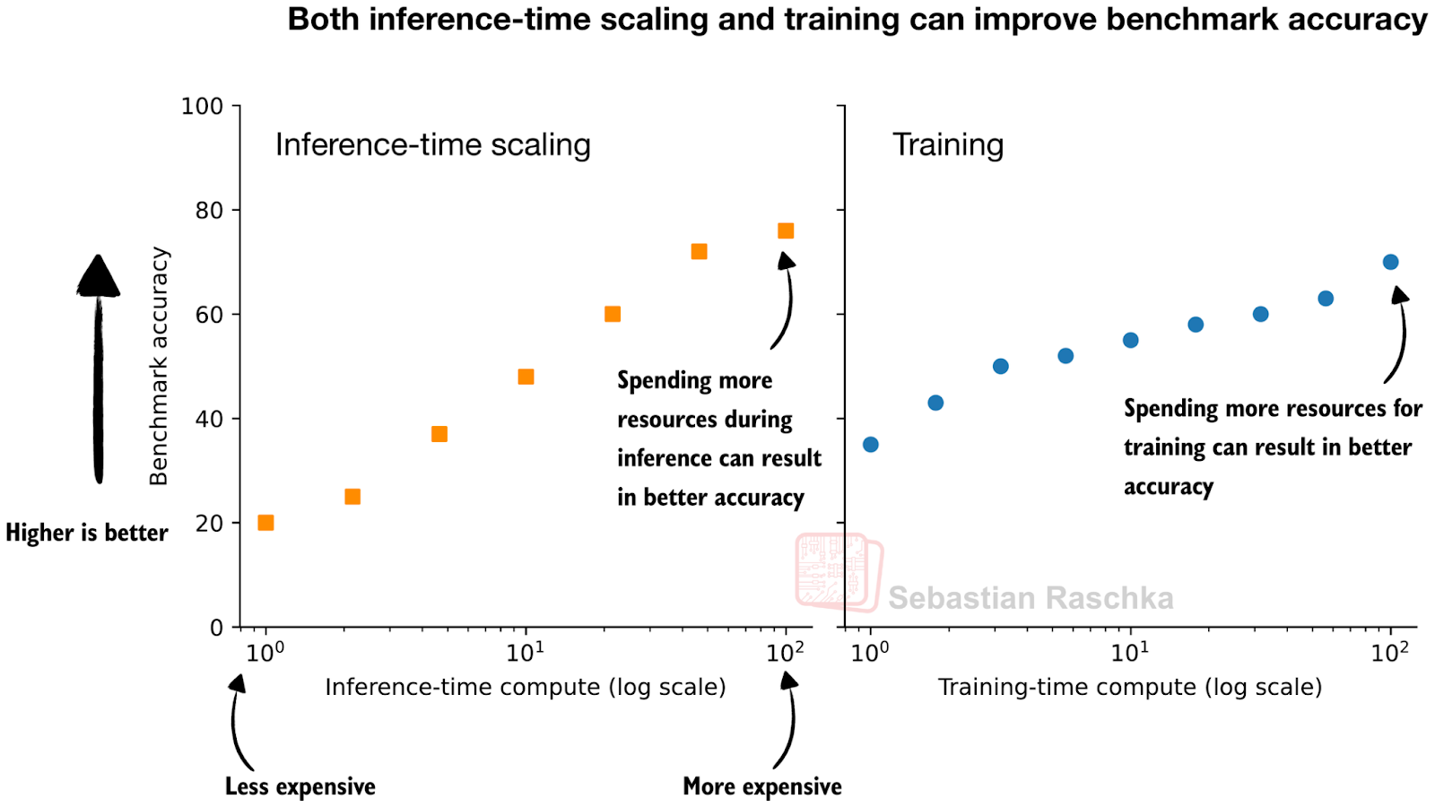
Two routes to higher benchmark accuracy. Left: holding the model fixed and spending more compute at inference time. Right: spending more compute during training to produce a stronger model. This section studies the left-hand curve for kernel generation; Section 3 studies the right (credit: Sebastian Raschka).
Kernel generation is an unusually good fit for inference-time scaling, for one structural reason: it has a cheap, automatic verifier. Compiling a kernel, checking its output against a reference, and timing it is fully automated, so unlike open-ended text generation, we can always keep the best verified candidate out of however many we produce. That single fact is what makes spending more compute pay off, and it is also what makes the verifier the true bottleneck, as the last part of this subsection argues and Section 2.3 develops in full.
Three axes of test-time compute #
Test-time compute can be spent along three axes, and every system in this section is one choice among them:
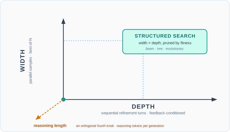
Test-time compute spent along three axes. Width (vertical) draws parallel samples; depth (horizontal) refines one trajectory over feedback turns; structured search sits in the corner where both are high, combining width and depth and pruning by fitness (Section 2.2). Reasoning length is an orthogonal fourth knob: how many tokens the model emits per generation.
- Width (parallel sampling). Draw \( N \) independent kernels from the same prompt and return the best verified one (Best-of- \( N \) ). The more you draw, the likelier some sample is correct [1].
- Depth (sequential refinement). Spend the budget refining one trajectory over turns, each conditioned on execution feedback. This is the inference-time face of multi-turn, agentic refinement; the RL that trains a policy to do it well is developed in Section 3.3.
- Structured search. Combine width and depth: maintain several candidates, refine them, and prune by fitness. Beam search, tree search, and evolution (Section 2.2) all live here.
A fourth, orthogonal knob is the reasoning length per generation: how many chain-of-thought tokens the model emits before committing to code. We treat it separately below because, for kernels, more is not always better.
The general lesson from test-time-compute research is that how the budget is spent matters as much as how much: allocating compute optimally (choosing between more samples and more refinement based on difficulty) can beat naively scaling either axis, and can even substitute for a larger model [2, 3]. The rest of this subsection instantiates that lesson for kernels.
Width: parallel sampling and Best-of-N #
The simplest scaling is to sample many kernels and keep the fastest correct one. MKEvolve’s Parallel Scaling baseline does exactly this, drawing 160 independent kernels per problem [4], and it is the standard reference point every other method is measured against. Its behavior exposes both the appeal and the limit of pure width.
The appeal is coverage, the chance that at least one sample is correct. On MultiKernelBench [5], a multi-platform benchmark of 285 tasks across CUDA, AscendC (Huawei NPU), and Pallas (TPU), the best model under greedy one-shot decoding solves only 164 of 855 platform-task instances, but moving to
\( N = 5 \)
sampled generations raises Claude Sonnet 4 to 200 total passes, with CUDA Pass@5 reaching 55.8% [5]. ConCuR [6] shows the same lift on KernelBench, reported with the
\( \text{Fast}_p \)
metric: the fraction of problems solved with a kernel at least
\( p \)
times as fast as torch.compile. Going from Pass@1 to Pass@10, its KernelCoder-32B model rises from 58% to 91% executable and from 17% to 32%
\( \text{Fast}_1 \)
on Level 1, and from 59% to 95% executable on Level 2 [6]. More draws find more correct kernels.
The limit is that width has diminishing and uneven returns. On MultiKernelBench the same models that reach 47% CUDA Pass@1 manage only single-digit rates on AscendC and Pallas no matter how they are decoded, because the base model was barely exposed to those backends during training [5], and no amount of sampling conjures a capability the policy lacks. Width raises coverage but not the ceiling, which is why the systems below invest in depth and search instead. A cautionary corollary appears in robust benchmarking: because each additional sample is another chance to stumble onto an evaluator exploit, pure width amplifies reward hacking, which we return to below.
Parallel sampling is also the natural substrate for the population methods of Section 2.2. A beam search’s per-round expansion, or an evolutionary generation’s offspring, is a batch of parallel samples that is then pruned by fitness rather than merely deduplicated, which is what lets structured search convert raw width into directed progress [7].
Depth: sequential refinement #
The alternative to sampling wide is refining deep: spend the budget on successive turns of one trajectory, each reading the compiler error, correctness diff, or profile of the last. A kernel engineer works this way, compile, read the error, profile the result, revise, and an agent given the same tools does too, so depth is the inference-time analogue of that loop: the model emits a kernel, the environment runs it and returns feedback, and the next turn is conditioned on that feedback rather than starting from scratch. Its power is that it reuses information a fresh sample throws away; its cost is a growing context and the question of which turn actually earned the final reward, the two issues that make training a policy to refine well a problem in its own right (Section 3.3). The central empirical finding, from Kevin [8], is that under a fixed compute budget, investing in iterative refinement across turns outperforms drawing the same number of independent single-shot samples, because feedback is more informative than one-shot diversity [8]. Depth uses information that width discards.
Depth is not automatically better, though: it needs the feedback to be trustworthy and representative. Astra [9] makes this concrete by decomposing refinement into separate testing, profiling, planning, and coding agents that share a trajectory log over 5 rounds; the multi-agent form reached 1.32x average speedup on production SGLang CUDA kernels versus 1.08x for an otherwise identical monolithic agent, and the monolith even regressed to a slowdown on one kernel when unrepresentative test inputs biased its profiling [9]. Deeper refinement amplifies whatever the feedback says, so a bad measurement compounds.
Structured search: width times depth #
Real systems rarely pick a single axis; they combine them and let a fitness function prune. KernelEvolve [10] illustrates the pattern explicitly with a two-phase schedule: a draft phase (roughly the first 10 steps) of independent parallel sampling without feedback, followed by a tree-expansion phase (steps ~10 to 50) where each node ingests execution feedback and the search deepens under a selection policy (greedy, MCTS with UCT, or evolutionary) [10]. Width seeds diversity; depth then exploits the best seeds. This is the same width-times-depth structure as the beam searches of Section 2.2 (Autocomp, AccelOpt), and MKEvolve’s topology evolution [4], differing only in what gets pruned and what memory persists across steps.
The payoff of structuring the search, rather than scaling one axis blindly, is efficiency. MKEvolve reaches better kernels than a 160-sample beam search while spending 15% to 35% fewer LLM tokens, precisely because refining subkernels concentrates compute where it helps instead of regenerating whole kernels [4]. AccelOpt [11] makes the cost argument even sharper: open-source models running its search-plus-memory loop matched Claude Sonnet 4 kernel quality at roughly 26x lower cost [11]. Well-structured search converts a fixed compute budget into more improvement per token.
The reasoning-token axis: more is not always better #
Reasoning models spend test-time compute a fourth way, by emitting long chains of thought before the code. It is tempting to assume longer reasoning yields better kernels, but the kernel evidence points the other way. ConCuR [6] measured it directly and found that shorter correct reasoning traces correlate with higher kernel-generation accuracy, while speedup is essentially uncorrelated with reasoning length (Pearson \( r \approx -0.047 \) ) [6]. Curating training data toward the shortest correct-and-fast trace per problem, just 4,892 examples, produced an open-source model competitive with far larger reasoning models on KernelBench [6]. The token budget is better spent on width or depth of search than on length of monologue.
Reasoning length is still useful as a difficulty signal. ConCuR proposes Average Reasoning Length as a per-task difficulty metric (Easy under 4000 tokens, Medium 4000 to 8500, Hard above), which is exactly the kind of estimate an inference-scaling controller needs to allocate its budget: sample wider and refine deeper on the tasks a difficulty proxy flags as hard, and stop early on the easy ones [6]. This closes the loop back to the “compute-optimal allocation” idea [2]: the win is not more compute everywhere, but more compute where it moves the needle.
Verification is the enabler and the bottleneck #
Every axis above rests on the same foundation: a verifier good enough that “the best of \( N \) ” or “the fittest survivor” actually is the best kernel. Scaling inference compute scales the search’s contact with that verifier, so any gap in it is found and exploited faster the harder we search: the more candidates we generate, the more likely one of them games the check rather than solving the task. This is reward hacking, and because it is the failure mode that all of the axes above share, the next-but-one subsection (Section 2.3) is devoted to it: the taxonomy of how kernels cheat a checker, the verification pipeline that catches them, and the anti-cheating benchmarks that keep measured speedups honest. Here we only sketch why it is inseparable from scaling.
The robust-kbench study [7] quantifies the danger. On benchmark tasks with exploitable evaluators, generated kernels reported fake speedups as large as 50x to 120x (for example by hardcoding a softmax output to 1.0), and after excluding the contaminated tasks the average measured speedup collapsed from 3.13x to 1.49x [7]. Its defenses are exactly what inference-time scaling needs to stay honest: cheap LLM verifiers that reject bad kernels before expensive hardware runs, plus anti-cheating filters (diverse initializations, multiple input configurations, forward and backward passes, and rejection of degenerate near-constant outputs) [7]. FlashInfer-Bench [12] adds the deployment-grounded version, scoring candidates on real serving traces and injecting the winner into a live SGLang or vLLM engine so the measured speedup is end-to-end rather than an isolated micro-benchmark [12].
This is why the benchmarks themselves are load-bearing for inference-time scaling, not incidental. Each one hardens a different failure mode of “just search harder”:
- KernelBench [13] defines the core protocol, correctness within tolerance plus the
\( \text{Fast}_p \)
speedup metric over
torch.compile, that the systems in this section report against. - MultiKernelBench [5] extends it across three hardware backends, exposing that search gains on CUDA do not transfer to under-represented backends without more than sampling.
- robust-kbench [7] closes the correctness and timing loopholes that scaled sampling would otherwise exploit (Section 2.3).
- FlashInfer-Bench [12] grounds evaluation in production LLM-serving workloads and live substitution, so the search optimizes what actually ships.
The through-line of this subsection, and of the section, is that inference-time compute buys better kernels only in proportion to how trustworthy the verifier is. Width, depth, search, and reasoning length are all levers on the same machine, and a leaky evaluator turns every one of them into a lever for cheating rather than for speed.
Takeaways #
- Inference-time scaling trades test-time compute for kernel quality along three axes, width (parallel Best-of- \( N \) ), depth (sequential, feedback-conditioned refinement, whose training is Section 3.3), and structured search (beam/tree/evolution, Section 2.2), plus an orthogonal reasoning-length knob.
- Width raises coverage cheaply but not the capability ceiling and has uneven, diminishing returns; depth exploits feedback that width discards but amplifies bad measurements; structured search combines both and, when well-organized, reaches better kernels for fewer tokens (MKEvolve’s 15-35% saving, AccelOpt’s 26x cost cut).
- For kernels, longer reasoning is not always better (shorter correct traces correlate with higher accuracy, and speedup is uncorrelated with trace length); reasoning length is better used as a difficulty signal for compute-optimal budget allocation.
- All of it depends on a trustworthy verifier: scaling search scales exposure to evaluator exploits, so the verification pipeline and anti-cheating benchmarks (robust-kbench, FlashInfer-Bench) of Section 2.3 are what let inference-time compute buy real speed instead of reward hacking.
References #
- B. Brown, J. Juravsky, R. Ehrlich, R. Clark, Q. V. Le, C. Ré, and A. Mirhoseini. Large Language Monkeys: Scaling Inference Compute with Repeated Sampling. arXiv:2407.21787, 2024. arxiv.org/abs/2407.21787
- C. Snell, J. Lee, K. Xu, and A. Kumar. Scaling LLM Test-Time Compute Optimally Can Be More Effective Than Scaling Model Parameters. arXiv:2408.03314, 2024. arxiv.org/abs/2408.03314
- NVIDIA Developer Blog. Automating GPU Kernel Generation with DeepSeek-R1 and Inference-Time Scaling. 2025. developer.nvidia.com/blog/automating-gpu-kernel-generation-with-deepseek-r1-and-inference-time-scaling
- J. Yoo, R. Saha, S. Zhu, T. Yu, W. Tang, and Y. Park. MKEvolve: A Modular Multi-Agent Framework for Kernel Code Generation. arXiv:2607.20501, 2026 (ICML 2026 Workshop on Compositional Learning). arxiv.org/abs/2607.20501
- Z. Wen, Y. Zhang, Z. Li, Z. Liu, L. Xie, and T. Zhang. MultiKernelBench: A Multi-Platform Benchmark for Kernel Generation. arXiv:2507.17773, 2025. arxiv.org/abs/2507.17773
- L. Kong, J. Wei, H. Shen, and H. Wang. ConCuR: Conciseness Makes State-of-the-Art Kernel Generation. arXiv:2510.07356, 2025. arxiv.org/abs/2510.07356
- R. T. Lange, Q. Sun, A. Prasad, M. Faldor, Y. Tang, and D. Ha. Towards Robust Agentic CUDA Kernel Benchmarking, Verification, and Optimization. arXiv:2509.14279, 2025. arxiv.org/abs/2509.14279
- C. Baronio, P. Marsella, B. Pan, S. Guo, and S. Alberti. Kevin: Multi-Turn RL for Generating CUDA Kernels. arXiv:2507.11948, 2025. arxiv.org/abs/2507.11948
- A. Wei, T. Sun, Y. Seenichamy, H. Song, A. Ouyang, A. Mirhoseini, K. Wang, and A. Aiken. Astra: A Multi-Agent System for GPU Kernel Performance Optimization. arXiv:2509.07506, 2025. arxiv.org/abs/2509.07506
- G. Liao, H. Qin, Y. Wang, A. Golden, M. Kuchnik, et al. KernelEvolve: Scaling Agentic Kernel Coding for Heterogeneous AI Accelerators at Meta. arXiv:2512.23236, 2026. arxiv.org/abs/2512.23236
- G. Zhang, S. Zhu, A. Wei, Z. Song, A. Nie, Z. Jia, N. Vijaykumar, Y. Wang, and K. Olukotun. AccelOpt: A Self-Improving LLM Agentic System for AI Accelerator Kernel Optimization. arXiv:2511.15915, 2025. arxiv.org/abs/2511.15915
- S. Xing, Y. Zhai, A. Jiang, Y. Dong, Y. Wu, Z. Ye, C. Ruan, Y. Huang, Y. Zhang, L. Yin, et al. FlashInfer-Bench: Building the Virtuous Cycle for AI-driven LLM Systems. arXiv:2601.00227, 2026. arxiv.org/abs/2601.00227
- A. Ouyang, S. Guo, S. Arora, A. L. Zhang, W. Hu, C. Ré, and A. Mirhoseini. KernelBench: Can LLMs Write Efficient GPU Kernels? ICML 2025. openreview.net/forum?id=yeoN1iQT1x