Reinforcement Learning from Execution Feedback #

Section 3.1 left us with an SFT model that is grounded in a kernel language (it produces valid, idiomatic code) but capped by imitation: it can only reproduce the corpus it was shown, with no way to tell a fast kernel from a merely reference-like one. Closing that gap is the job of this section. The reason it needs a new tool is that writing a kernel that is fast on a specific piece of hardware is a different problem from writing one that is merely valid. Performance is governed by low-level, device-specific decisions: memory-hierarchy staging, tiling and block sizes, occupancy, coalesced access, tensor-core utilization. The only faithful measure of whether those decisions are good is to run the kernel and time it. A model trained purely to reproduce plausible-looking code has no access to that signal and no objective that rewards it, so it plateaus at “valid but not hardware-optimized.”

Reinforcement learning (RL) is the tool that optimizes this missing objective directly. Instead of imitating a fixed corpus of code, we let the model generate kernels, run them on the target hardware, and learn from the outcome: kernels that compile, produce correct results, and run faster are reinforced, while those that fail are discouraged. Kernels are an especially favorable setting for this. Unlike open-ended language tasks, they come with an automatic, high-fidelity oracle: compile the kernel, check it against a reference, and time it on hardware. The reward is therefore verifiable and objective rather than a learned proxy, the regime known as RL with verifiable rewards (RLVR). This makes RL cheaper and more reliable for kernels than for domains that hinge on human-preference models, and is why RL post-training has become the dominant recipe for state-of-the-art kernel generators. Building on the general RL post-training machinery of Section 1.6 (the objective, policy gradients, and the PPO and GRPO algorithms), this subsection focuses on what is specific to kernels: casting kernel generation as an RL problem and describing the execution-feedback loop that turns a compiler and the hardware into a reward signal.

Example: RL workflow for kernel optimization #

Before diving into the pieces, here is the overall loop: RL post-training for kernels is an iterative cycle built from four ingredients: a pool of tasks, a policy, a reward computed by execution, and a policy-gradient optimizer:

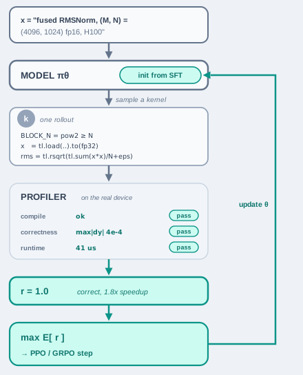
The execution-feedback loop. A sampled task is turned into candidate kernels by the policy; the profiler executes each one, compile · check · time, into a verifiable reward; a policy-gradient step then reinforces the fast, correct kernels, and the cycle repeats.

Each step of the loop: (1) sample a task from the data pool; (2) the policy (initialized from the SFT model of Section 3.1) generates one or more candidate kernels, optionally over several refinement turns; (3) each kernel is run in a sandboxed environment that returns a verifiable reward from compilation, correctness, and speed; (4) a policy-gradient algorithm (PPO or GRPO) nudges the policy toward the higher-reward kernels. Repeating this cycle is what drives the policy past the “valid but not hardware-optimized” plateau.

A concrete pass. Take the RMSNorm task from Section 3.1 as \( x \) . The policy emits a candidate kernel \( y \) and the sandbox then (i) compiles it (a build failure ends the pass with a low reward); (ii) checks correctness by running \( y \) on held-out test inputs and comparing its output against the PyTorch reference within numerical tolerance; and (iii) times it against that reference to get a speedup. A kernel that compiles, matches the reference, and runs 1.8× faster earns a high reward and is reinforced; one that computes the wrong thing (say, LayerNorm) or is correct but slower is penalized. Over many such passes the policy shifts toward kernels that are both correct and fast.

The sandbox that produces this reward is a piece of infrastructure worth designing deliberately, because it executes untrusted, model-generated code on real accelerators:

• Isolation. Each candidate runs in a separate process (or container) with a hard timeout and memory cap, so a kernel that hangs, deadlocks, or corrupts device state cannot stall or crash training; it is simply killed and scored as a failure.
• Determinism and fairness. Correctness is checked against fixed test inputs at a set tolerance, and timing uses warm-up runs plus repeated trials (reporting, e.g., the median) on a pinned hardware target, so the speedup signal is reproducible rather than noisy. TritonRL [2], for instance, grades correctness on 5 random test inputs and takes each kernel’s runtime as the mean of 10 timed runs.
• Throughput. Because RL needs a reward for every rollout, the sandbox is typically pooled across many workers/devices and caches compilation. In practice the throughput of this environment, not the policy update, is often what limits training, so building a robust distributed kernel environment (for example Dr. Kernel’s KernelGYM [3]) is an engineering contribution in its own right.

In the multi-turn and agentic settings (Section 3.3), this same environment is exposed to the policy as callable tools (a compiler, a runner, a profiler), so kernel RL doubles as an instance of tool-use RLVR, with the tools’ output serving as both the model’s feedback and the source of the reward.

The rest of this subsection expands each ingredient in turn: the data that defines the tasks (next), the RL formulation specialized to kernels (building on the algorithms of Section 1.6), the reward computed from execution feedback, the curriculum that decides which tasks to train on, and the multi-turn setting that lets the policy revise using feedback.

Data #

Unlike SFT, where every task should be paired with an expert kernel to imitate, RL needs no reference kernels. An example is just a task: an operator specification together with a reference implementation (e.g., the PyTorch function) and test inputs. The reward comes from running the model’s own kernel and checking it against that reference, not from comparing it to a stored expert solution. This sharply lowers the data barrier: any operator for which a slow but obviously-correct reference can be written is a usable RL task, even if no fast kernel for it exists anywhere.

Whereas SFT trained on labeled pairs \( \mathcal{D} = \{(x^{(i)}, y^{(i)})\} \) (Section 3.1), an RL task set carries no target kernels; each element is just a prompt \( x^{(i)} \) :

and the kernels \( y \sim \pi_\theta(\cdot \mid x) \) are produced at training time rather than stored. The prompt \( x \) itself can take several forms depending on how much scaffolding the task provides: from a plain natural-language description of the desired function, to an instruction alone, to an instruction plus a reference implementation, to an instruction plus a reference plus a seed kernel to optimize. The only firm requirement is that \( x \) admit an automatic correctness and performance check (usually via a reference implementation and test inputs), since that check is what produces the reward. Concretely, the RL task for our running RMSNorm example is just the Section 3.1 prompt, without the target kernel:

Task x:
  Write a Triton kernel that computes fused RMSNorm over the last dimension,
  for x of shape (M, N), fp16, on NVIDIA H100.
  Reference (PyTorch):
      def rmsnorm(x, w, eps=1e-6):
          rms = x.pow(2).mean(dim=-1, keepdim=True).add(eps).rsqrt()
          return x * rms * w
  Test inputs: (M, N) in {(4096, 1024), (8192, 4096), ...}, random fp16.

Compare this with the SFT pair in Section 3.1: there the reference Triton kernel was the target \( y \) the model was trained to reproduce; here there is no \( y \) at all. The rmsnorm reference and the test inputs are the entire task, and together they are the reward oracle: the sandbox runs the model’s kernel on the test inputs and grades it against rmsnorm for correctness and speed.

Several public sources supply such tasks:

• KernelBench [12]: a few hundred PyTorch reference modules organized by difficulty level; serves as both the standard evaluation benchmark and a common task source.
• TritonBench [13]: a large set of real-world Triton operators.
• KernelBook [14]: many PyTorch–Triton pairs whose PyTorch side alone already furnishes RL tasks (its Triton side is needed only for SFT).
• CUDA-Agent-Ops-6K [15]: ~6,000 synthesized operator-level CUDA tasks (fused compositions of PyTorch operators), filtered and decontaminated against KernelBench (CUDA Agent [4]).

Beyond these fixed datasets, tasks can also be synthesized programmatically, composing primitive operators into fused programs at controlled difficulty, which is how CUDA-Agent-Ops-6K above was built and how several curriculum methods obtain broad, difficulty-labeled coverage (CUDA Agent [4]; DRTriton [5]).

Because the reference and test inputs are the reward oracle, a task is only as good as that check, and its quality directly bounds the training signal:

• A trustworthy reference. The reference must be unambiguously correct (even if slow), since every generated kernel is graded against it; a buggy reference wrongly rewards kernels for being wrong.
• Representative, adversarial test inputs. Correctness is only ever checked on the provided inputs, so they must exercise the shapes, dtypes, and edge cases that matter (e.g., non-power-of-two N, tail masking, extreme values). Thin or too-forgiving tests are exactly what let a model reward hack, passing the check without implementing the operator (Section 2.3), so the tests double as the corpus’s integrity guarantee. Rather than hand-write them, systems often synthesize several input configurations per task and keep only those that execute correctly against the reference; TritonRL [2] generates varied input shapes this way and reports better robustness to unseen shapes as a result.
• A meaningful performance baseline. The speed reward is relative to a baseline (the PyTorch reference, or an existing kernel to beat), so a fair, well-tuned baseline is what makes “faster” mean something rather than rewarding a kernel for merely outrunning an artificially slow reference.

RL formulation for kernels #

The generic RL machinery, the expected-reward objective \( J(\theta) = \mathbb{E}_{x\sim\mathcal{D}}\,\mathbb{E}_{y\sim\pi_\theta(\cdot\mid x)}[\,r(x,y)\,] \) , its optimization by policy gradients, and the PPO and GRPO algorithms that carry out the update, is developed in Section 1.6. Here we take that formulation as given and focus on what is specific to kernels: the policy is our SFT model \( \pi_\theta(y \mid x) \) that maps a task prompt \( x \) (operator specification, reference implementation, hardware target) to a candidate kernel \( y \) , and the reward \( r(x, y) \) is obtained by executing that kernel (compile + correctness + performance).

Two properties of this reward shape everything downstream:

• It is terminal and sparse. \( r(x, y) \) is defined only once the entire kernel has been generated, compiled, and run. There is no meaningful way to score a half-written kernel, so no intermediate per-token rewards exist. A whole kernel therefore earns a single scalar that must be attributed back across the hundreds of token-level actions that produced it, ideally separating the tokens that encoded a good tiling or fusion decision from those that merely completed boilerplate. In plain policy-gradient training this scalar is applied uniformly to every token of the rollout (Section 1.6), so attribution happens only in aggregate over many samples; sharper credit assignment (per-turn or per-token) is a distinct problem, taken up in Section 3.3.
• It is verifiable and deterministic. The reward comes from an objective checker (a compiler and a profiler), not a learned preference model, and the same kernel graded the same way yields the same score, up to timing noise the sandbox averages out. This is exactly the RLVR regime, and it is what makes RL cheaper and more reliable for kernels than for open-ended language tasks.

The pay-off of this formulation is the same one that motivated the section: unlike SFT, which minimizes a divergence to a fixed dataset, RL maximizes reward over the policy’s own samples, so it can reinforce a correct, fast kernel the model discovered on its own, even one that appears in no reference corpus, and thereby surpass its teacher.

Why GRPO fits kernels. Of the two algorithms, GRPO is the workhorse of modern kernel RL (used by AutoTriton [1], TritonRL [2], DRTriton [5], and others), and its group-relative baseline is a natural match: sampling several candidate kernels for the same operator and rewarding the ones that run fastest relative to their siblings is a direct, low-overhead comparison, with no value network to train (a real saving when the policy is already a multi-billion-parameter model). It does, however, sharpen a kernel-specific failure mode: when every kernel in a group earns the same reward (e.g., all fail to compile early in training), the group-relative advantage is zero and the task yields no gradient, which is exactly what the curriculum and task-selection strategies below are designed to avoid.

Rewards from execution feedback #

The reward is returned by the environment: executing a candidate kernel yields the three signals it is built from, namely whether the kernel compiles, whether it is correct against the reference, and how fast it runs (its runtime, and the speedup over a baseline). The rest of this section turns those signals into a scalar.

The most basic execution-based reward is simply binary correctness: in settings such as math or coding, the environment returns 1 when the generated answer is verified correct (the right final answer, or all unit tests passing) and 0 otherwise,

For kernels, though, the environment returns far more than a pass/fail bit: the profiler exposes runtime, memory-bandwidth utilization, occupancy, and where the time is spent. This richer feedback lets us build a more fine-grained reward that scores not only correctness but how fast and how efficient the kernel is.

Putting the three checks together, a kernel reward is gated: compilation is a prerequisite for any correctness credit, and correctness for any performance credit. Schematically,

with \( r_{\text{compile}} \le r_{\text{incorrect}} \le 0 \) penalizing the two failure modes and \( f \) a monotonically increasing function of the measured speedup over a baseline,

where \( t(x, y) \) is the runtime of the generated kernel and \( t_{\text{ref}}(x) \) that of the baseline (the reference implementation, or an existing kernel to beat). The gating is what stops the policy from being paid for a fast-but-wrong kernel. Production systems often add a further outer gate on top of compilation and correctness: TritonRL [2], for instance, multiplies both reward branches by a validity check (syntax plus a functionality test that the code is a genuine Triton kernel rather than a wrapper around a framework op) and bounds the speed term with a clip at \( 2\times \) , so a kernel earns speed credit only once it is valid and correct, and no single extreme measurement can dominate. The exact choice of \( r_{\text{compile}} \) , \( r_{\text{incorrect}} \) , and \( f \) is the reward-design question of Section 3.4, and the reward-hacking pitfalls it opens up are the subject of Section 2.3.

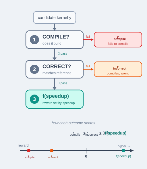
The gated reward. Compilation gates correctness, which gates performance: a kernel that fails to build scores \( r_{\text{compile}} \) , one that builds but is wrong scores \( r_{\text{incorrect}} \) , and only a compiled-and-correct kernel is paid by speed via \( f(\mathrm{speedup}) \) (highlighted). The number line shows the resulting ordering \( r_{\text{compile}} \le r_{\text{incorrect}} \le 0 < f(\mathrm{speedup}) \) , so no fast-but-wrong kernel can ever outscore a correct one.

Whatever its granularity, the reward must align with the true objective of the task. RL optimizes exactly the scalar it is handed: the policy converges toward the optimal policy for the reward, which matches the kernel we actually want only if the reward faithfully captures it. A misaligned reward, one that scores a fast-but-slightly-wrong kernel highly, or one a kernel can appear to satisfy without genuinely being fast, is a proxy the policy will learn to exploit rather than the goal we intended. Designing a reward that captures “correct and genuinely fast on the target hardware” is precisely what Section 3.4 addresses, and keeping the policy from gaming it is the subject of Section 2.3.

Curriculum and task selection #

Given a pool of tasks, the quality of RL then hinges on which of them the policy trains on and how they are sampled. This matters because the execution reward is sparse and coarse: early in training a weak policy may compile nothing (uniformly zero reward, no gradient), and even later a task is often all-or-nothing across a sampled group, and when every sample in a GRPO group earns the same reward, the group-relative advantage \( \hat{A}_i \) is exactly zero, so the task contributes no learning signal. To keep the policy on tasks in its learnable zone, where at least some sampled kernels succeed and yield a non-zero advantage, curriculum or task selection for RL is important.

This degeneracy is precise. GRPO centers each sample’s reward on its group mean to form the advantage (Section 1.6),

so if every sample in the group earns the same reward, \( r_1 = \dots = r_G \) , then \( r_i - \bar{r} = 0 \) for all \( i \) and the prompt contributes no gradient. A prompt is therefore informative only when its group has reward variance, \( \sigma_r \gt 0 \) . For a binary correctness reward this is simply

that is, the policy solves the task sometimes but not always. This band is exactly the “learnable zone”: trivially easy prompts ( \( \bar{p} = 1 \) ) and currently impossible ones ( \( \bar{p} = 0 \) ) both drop out of the gradient. Static curation aims the fixed training distribution at this band ahead of time; adaptive sampling (below) discards zero-variance groups on the fly.

To make this concrete, take a group of \( G = 4 \) kernels sampled for one prompt and scored by the gated reward above (say \( r_{\text{compile}} = -1 \) , \( r_{\text{incorrect}} = -0.5 \) , and \( f(\mathrm{speedup}) = \mathrm{speedup} \) ). Early in training all four might fail to compile, \( (r_1, \dots, r_4) = (-1, -1, -1, -1) \) : then \( \bar{r} = -1 \) , \( \sigma_r = 0 \) , every \( \hat{A}_i = 0 \) , and the prompt produces no gradient. Once the policy can sometimes succeed, the group might read \( (-1, -1, -0.5, 1.5) \) (two fail to compile, one is incorrect, one is correct at a 1.5× speedup): now \( \bar{r} = -0.25 \) and \( \sigma_r \gt 0 \) , so the fast correct kernel gets a positive advantage \( \hat{A} = (1.5 - (-0.25))/\sigma_r \gt 0 \) and is reinforced while the failures are pushed down. Curriculum and task selection exist to keep groups in this second regime.

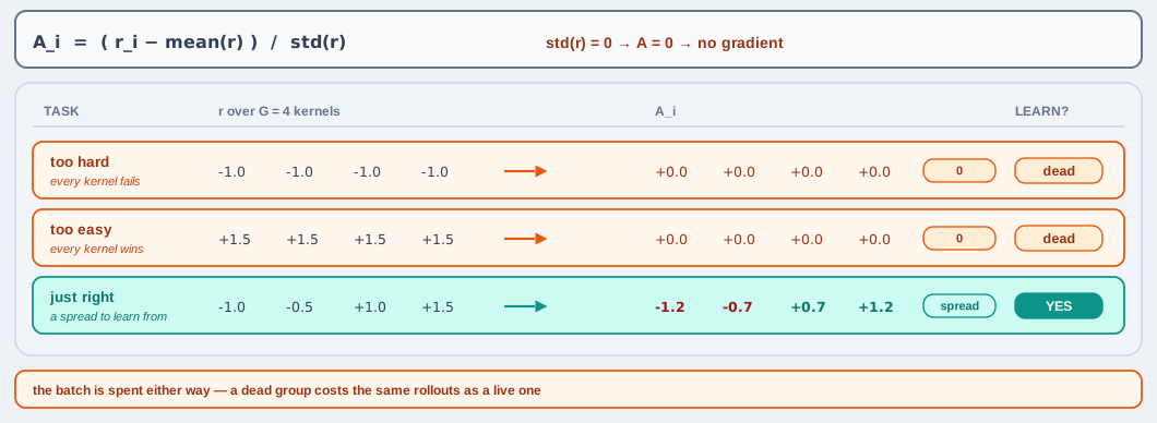
The zero-variance failure mode, for \( G = 4 \) . Both dead rows are worth noting: a task can be uninformative because it is too hard (every kernel fails) but equally because it is too easy (every kernel wins) — the normalization is blind to where the group sits, only to whether it spreads. Only the just-right row yields non-zero advantages, ranking its four kernels against each other. And the cost is symmetric: a dead group consumes exactly the same \( G \) rollouts as a live one, which is what makes the curation and adaptive-sampling machinery below worth its complexity.

Static curation #

Here the training distribution is fixed ahead of time, independently of the policy, by selecting or weighting tasks according to a difficulty estimate. That estimate can be intrinsic to the task (its operator count, or its category, a single-operator kernel versus a fused multi-operator one) or model-relative (how often a fixed base model already solves it); either way the goal is the same: concentrate the pool where the policy can actually learn. This shows up under a few familiar names: a curriculum that orders tasks easy-to-hard on a schedule, data mixing that fixes the proportions of easy versus hard categories, and difficulty filtering that drops tasks the base model almost always or never solves. Curriculum learning is a long-standing idea [7], and recent reasoning-RL systems apply it heavily to math and code, staging training from easy to hard (or from one domain to another) and filtering by the pass rate of a fixed model measured once offline (Light-R1 [8]; Skywork-OR1 [10]; and the code stage of AceReason-Nemotron [9]), with kernel-RL work following suit (DRTriton [5]; TritonRL [2]). TritonRL, for instance, uses an LLM labeler (Qwen3-235B-Instruct) to sort tasks into the KernelBench [12] tiers (single-operator, operator-fusion, full-architecture) and then, notably, finds that training its RL stage exclusively on the single-operator tier gives the best correctness and match-or-beat-reference rate on both single-operator and fusion evaluations: fusion tasks succeed so rarely that their groups are almost always zero-variance (above) and contribute little signal, while single-operator skill appears to transfer upward. The lesson is not that easy tasks are always better, but that a task earns its place in the mixture only while the policy still solves it sometimes, keeping its groups inside the learnable band.

Adaptive sampling #

The training distribution is instead shaped continuously, from the current policy’s own behavior. The canonical instance is dynamic sampling (DAPO [6]): at each step, groups whose completions are all-pass or all-fail carry zero advantage and are discarded, keeping only prompts that still produce a learning signal, so the effective difficulty band tracks the policy as it improves. Because the selection criterion, the policy’s success rate, is exactly the one used offline, adaptive sampling is essentially the online, per-step version of difficulty filtering: the same idea, recomputed every update instead of frozen into a fixed dataset. Reasoning-RL systems use this online form directly: prompts are filtered by the current model’s success rate at each step [11], and prompts the current model already solves too often are dropped mid-training (AceReason-Nemotron [9], for its math stage; its code stage instead filters offline with a fixed model, the static counterpart).

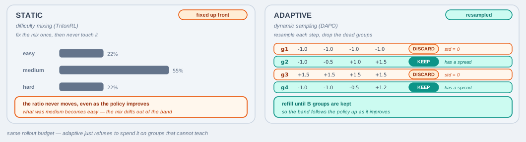
Static difficulty mixing fixes the easy/medium/hard proportions up front, so the mix drifts out of the learnable band as the policy improves; adaptive sampling discards the dead groups each step and refills, so the band tracks the policy.

In kernel RL, this online, advantage-based filtering remains uncommon, but the setting also admits a kernel-specific selection signal that generic text or math RL lacks. Instead of keeping a rollout because its group still has reward variance, one can prioritize it by how much of the end-to-end runtime the target operator accounts for (Dr. Kernel [3]). The intuition is Amdahl’s law: optimizing a kernel that consumes, say, 40% of a model’s runtime is far more valuable than one that consumes 0.5%, no matter how large its local speedup, so training compute is better spent on the dominant operators. This signal is essentially free here, because the environment already profiles every rollout to compute the reward, so per-operator timing is a by-product of scoring rather than extra work. Note this is a selection criterion (which tasks and rollouts to learn from), orthogonal to the reward itself; it can be combined with the advantage-based filtering above rather than replacing it.

Multi-turn RL and agentic refinement #

So far the policy gets one attempt per task: sample a kernel, run it, receive a terminal reward. But a human kernel engineer rarely writes a kernel once; they compile it, read the error, profile the result, and revise. Letting the policy act over several feedback-conditioned turns is multi-turn RL. Because it is the natural home for that material, we develop multi-turn RL (its trajectory objective, context management, and cross-turn credit assignment) in Section 3.3, alongside the single-turn baseline it extends.

References #

RL post-training for kernel generation.

1. S. Li, Z. Wang, Y. He, Y. Li, Q. Shi, J. Li, Y. Hu, W. Che, X. Han, Z. Liu, and M. Sun. AutoTriton: Automatic Triton Programming with Reinforcement Learning in LLMs. arXiv:2507.05687, 2025. arxiv.org/abs/2507.05687
2. J. Woo, S. Zhu, A. Nie, Z. Jia, Y. Wang, and Y. Park. TritonRL: Training LLMs to Think and Code Triton Without Cheating. arXiv:2510.17891, 2025. arxiv.org/abs/2510.17891
3. W. Liu, J. Xu, Y. Li, L. Zheng, T. Li, Q. Liu, and J. He. Dr. Kernel: Reinforcement Learning Done Right for Triton Kernel Generations. arXiv:2602.05885, 2026. arxiv.org/abs/2602.05885
4. W. Dai, H. Wu, Q. Yu, H. Gao, J. Li, C. Jiang, W. Lou, Y. Song, H. Yu, J. Chen, W. Ma, Y. Zhang, J. Liu, M. Wang, X. Liu, and H. Zhou. CUDA Agent: Large-Scale Agentic RL for High-Performance CUDA Kernel Generation. arXiv:2602.24286, 2026. arxiv.org/abs/2602.24286
5. S. Guo, M. Lin, and T. Yang. DRTriton: Large-Scale Synthetic Data Driven Reinforcement Learning for Triton Kernel Generation. arXiv:2603.21465, 2026. arxiv.org/abs/2603.21465

(The core RL objective and the PPO / GRPO algorithms are covered, with references, in Section 1.6. Multi-turn RL and its references are in Section 3.3.)

Curriculum and task selection.

6. Q. Yu, Z. Zhang, R. Zhu, et al. DAPO: An Open-Source LLM Reinforcement Learning System at Scale. arXiv:2503.14476, 2025. arxiv.org/abs/2503.14476
7. Y. Bengio, J. Louradour, R. Collobert, and J. Weston. Curriculum Learning. ICML, 2009. dl.acm.org/doi/10.1145/1553374.1553380
8. L. Wen, Y. Cai, F. Xiao, et al. Light-R1: Curriculum SFT, DPO and RL for Long CoT from Scratch and Beyond. arXiv:2503.10460, 2025. arxiv.org/abs/2503.10460
9. NVIDIA. AceReason-Nemotron: Advancing Math and Code Reasoning through Reinforcement Learning. arXiv:2505.16400, 2025. arxiv.org/abs/2505.16400
10. Skywork AI. Skywork Open Reasoner 1 Technical Report. arXiv:2505.22312, 2025. arxiv.org/abs/2505.22312
11. S. Bae, et al. Online Difficulty Filtering for Reasoning-Oriented Reinforcement Learning. arXiv:2504.03380, 2025. arxiv.org/abs/2504.03380

Datasets and benchmarks.

12. A. Ouyang, S. Guo, S. Arora, A. L. Zhang, W. Hu, C. Ré, and A. Mirhoseini. KernelBench: Can LLMs Write Efficient GPU Kernels? arXiv:2502.10517, 2025. arxiv.org/abs/2502.10517
13. J. Li, X. Han, et al. TritonBench: Benchmarking Large Language Model Capabilities for Generating Triton Operators. arXiv:2502.14752, 2025. arxiv.org/abs/2502.14752
14. S. Paliskara and M. Saroufim. KernelBook. Hugging Face Datasets (GPUMODE/KernelBook), 2025. huggingface.co/datasets/GPUMODE/KernelBook
15. ByteDance–Tsinghua SIA. CUDA-Agent-Ops-6K. Hugging Face Datasets (BytedTsinghua-SIA/CUDA-Agent-Ops-6K), 2026. huggingface.co/datasets/BytedTsinghua-SIA/CUDA-Agent-Ops-6K