Roofline Analysis #

When an algorithm is run on hardware, there are three dominant constraints:

1. How many floating-point operations the chip can perform per second ("OPs/sec")
2. How many bytes per second the chip (or system) can move in memory or across an interconnect ("bandwidth")
3. How much memory you have in total (on-chip, off-chip, network) to hold data.

A roofline model blends all of these to give upper and lower bounds on runtime: The time an operation takes cannot be less than the you’d get if you were just limited by compute. More precisely,

$$T_{\text{math}} = \frac{\text{Computation OPs}}{\text{Accelerator OPs/s}}, \hspace{3ex} T_{\text{comm}} = \frac{\text{Communication bytes}}{\text{Memory Bandwidth bytes/s}}$$

Clearly, an upper bound on the latency of any operation is given by $T_{\text{math}} + T_{\text{comm}}$. Moreover, usually computation can be overlapped with communication. With a perfect overlap, we get a lower bound on the latency of any operation/algorithm to be $\text{max}\left(T_{\text{math}}, T_{\text{comm}}\right)$.

If communication and computation overlap perfectly, then whenever $T_{\text{math}} > T_{\text{comm}}$, the hardware stays fully utilized – a compute-bound regime. But if $T_{\text{math}} < T_{\text{comm}}$, we enter a communication-bound regime, meaning some compute capacity goes unused while the system waits on data transfers.

This is often formalized in terms of Accelerator intensity, which is a characteristic of the accelerator, and Computation intensity, which is a function of an operation/algorithm. These are defined as:

$$\text{Accelerator intensity} = \frac{\text{Accelerator OPs/s}}{\text{Bandwidth bytes/s}}$$ $$\text{Computation intensity} = \frac{\text{Computation OPs}}{\text{Communication bytes}}$$

If an operations has high computation intensity, it will tend to be compute-bound (i.e., you’re spending lots of FLOPs per byte of data moved). If it has low intensity, it will tend to be communication or memory bound (you’re moving a lot of data for each FLOP).

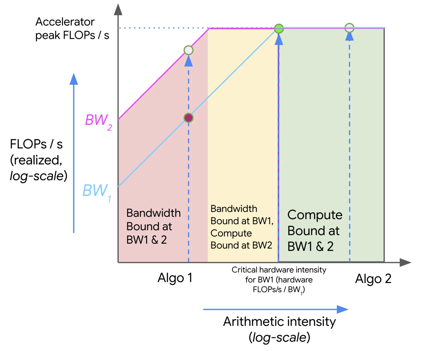
Visualization of roofline analysis (credits: How To Scale Your Model)

The plot above visualizes a roofline analysis. The X-axis corresponds to the computation intensity of any operation/algorithm, whereas the Y-axis is the achieved FLOPs/s of the operation on the hardware. The roofline itself is defined by two main limiting lines:

• A memory/communication-bandwidth bound line: For low computation intensity, performance is limited by how fast data can be moved (bytes/second) rather than how fast floating-point operations can be done.
• A compute-bound line: At high computation intensity, performance is limited by the peak FLOPs/sec of the hardware.

The intersection of these two types of limits defines a knee or critical intensity. In the figure above, two algorithms: Algo 1 and Algo 2, are plotted against two bandwidths (BW1 and BW2). The regions are color-coder (red = Bandwidth bound at both bandwidths, yellow = bandwidth bound only at the lower bandwidth, green = compute bound at both bandwidths).

Here’s how we can interpret the plot:

• If our algorithm lies to the left of the knee (i.e., low intensity), we are in the bandwidth/communication-bound regime. In this region, reducing bytes moved, increasing data reuse, improving memory locality, or boosting bandwidth, will improve performance more that increasing raw compute. The FLOPs/s achieved is significantly below the hardware peak.
• If our point lies to the right of the knee (i.e., high intensity), we are in the compute-bound regime. Here, we are hitting the hardware’s peak FLOPs/s (or close to it). Further increasing arithmetic intensity or bandwidth helps only marginally, as we are essentially limited by compute. Further gains require more compute capacity (or new precision formats, etc.)
• The slope of the left part of the plot (bandwidth-bound region) is linear in log-log space, i.e., performance increases with computation intensity (more FLOPs per byte = better). Once we hit the knee, the plot flattens because we cannot exceed peak compute.

Such a visualization gives us a quick, intuitive way to answer: Will our algorithm be limited by data movement or compute? and What do we need to optimize to get more performance?. Note: In distributed setups, the communication part of the roofline includes the inter-chip links, and thus the knee might shift (because inter-chip bandwidth is often lower than on-chip memory bandwidth). The roofline visualization extends to those cases too.

References #

1. All About Rooflines, How To Scale Your Model. https://jax-ml.github.io/scaling-book/roofline/