Mixture of Experts #

Scaling Laws for modern LLMs dictate that increasing the model size benefits generalization. A dense model with $N$ parameters executes all parameters per forward pass – making inference linearly more expensive as models scale in size.

The Mixture-of-Experts (MoE) architecture decouples model size from compute by activating only a small, routed subset of parameters per token. A model might store $1\text{T}$ parameters, yet compute on only a small fraction of parameters ($10-20\text{B}$) per token. This provides:

Higher parameter count $\implies$ Better quality of output
Lower per-token FLOPs $\implies$ Cheaper inference
Better scaling with parallel hardware (experts can be sharded across devices)

This trade-off makes MoEs fundamentally appealing for high-throughput inference. MoE modules are considered sparse because only a small subset of experts is activated for each input, unlike dense layers that always engage all parameters. At the same time, the large aggregate parameter count substantially increases the model’s capacity, allowing it to absorb more knowledge during training. This sparsity preserves inference efficiency, since only a fraction of the parameters are used at any given step.

MoE architecture overview #

An MoE layer replaces the standard feedforward network (FFN) block in a transformer. Instead of one FFN layer, we have $E$ experts, each of which is an independent MLP. This is demonstrated below:

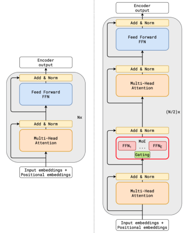
MoE layers replace standard FFN layers. MHA modules are remain unchanged (credits: Lepikhin et. al.)

In the figure above, every alternate transformer block has an MoE layer.

Routing #

For each input token representation $h \in \mathbb{R}^d$, a lightweight gating function first computes the scores:

$$g = W_gh, \quad \text{where} \quad W_g \in \mathbb{R}^{E \times d}.$$

Next, it selects the top-$k$ experts (typically $k = 1$ of $k = 2$), and routes the token’s hidden state to those experts. Formally,

$$G(h) = \text{Softmax}\left(\text{TopK}(g,k)\right).$$

Here, $\text{TopK}(g,k) = g_i, \text{if } g_i \text{ is in the top-k elements}, -\infty \text{ otherwise}$. Subsequently,

$$\text{MoE}(h) = \sum_{i = 1}^nG(h)_i E_i(h), \text{ where } E_i(h) \text{ is the output of expert } i.$$

Note that each selected expert proceses on the tokens routed to it. Experts operate in parallel across acelerator shards. The outputs are combined using the gating weights. The above computation is visualized below:

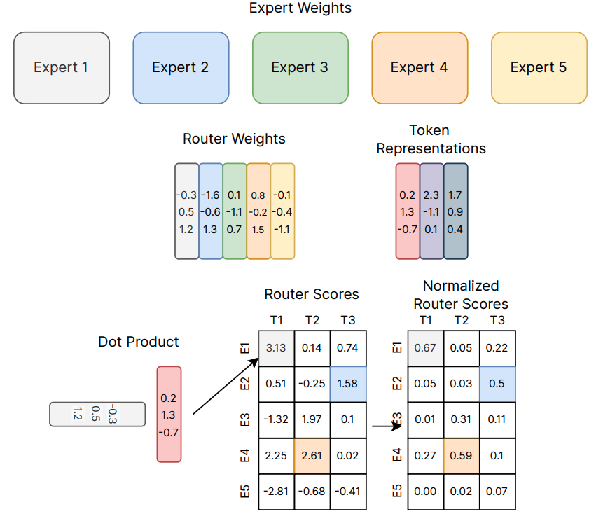
MoE layer computation (credits: Fedus et. al.)

Shared expert and Expert count #

Shared experts are a small but important design choice in many modern MoE models. They exist alongside the usual routed (sparse) experts and are invoked for every token, regardless of routing decisions. Similar to a dense feedforward block, shared experts are always active and process all tokens, guaranteeing a baseline capacity of the LLM. The DeepSpeed-MoE paper noted that having a shared expert boosts overall modeling performance compared to no shared expert. With a shared expert, the output is:

$$\text{MoE}(h) = E_{\rm shared}(x) + \sum_{i = 1}^nG(h)_i E_i(h)$$

A central design choice in MoE models is whether to allocate capacity as many small experts or fewer large experts, even when the total parameter budget is similar. This affects the inference efficiency and the parallelism technique chosen.

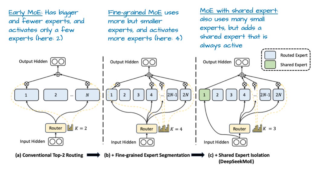
An annotated figure from DeepSeekMoE (borrowed from Sebastian Raschka)

Why MoE improves inference efficiency #

A transformer FFN (dense or expert MLP) typically consists of three linear layers: Gate projection $W_{\text{gate}} \in \mathbb{R}^{d \times f}$, Up projection $(W_{\text{up}} \in \mathbb{R}^{d \times f})$ (sometimes fused with the gate matrix), and Down projection $(W_{\text{down}} \in \mathbb{R}^{f \times d})$/. These projections expand the hidden dimension from $d$ to a larger dimension $f$, apply a non-linear activation (e.g., SiLU or GELU), then contract back. The expansion ratio $(r)$, i.e., $f/d$ refers to how much the hidden dimension expands inside the FFN relative to the model dimension.

Since the FFN cost is dominated by the matmuls $d \times f$ (gate, up) and $f \times d$ (down), the compute FLOPs scales as $\mathrm{O}\left(3rd^2\right)$. For an MoE with $E$ experts, top-$k$ routing has $\mathrm{O}\left(3krd^2\right)$ FLOPs per expert. Since we invoke a fixed number of experts ($k$ per token – for e.g., $k = 1$), the compute per token stays constant, even as $E$ increases, allowing models size to scale without scalig compute. In other words, the number of activated parameters during inferences tays fixed, even though the total model size can scale up.

Memory trade-off: Since all experts’ weights need to be stored, this increases VRAM usage as expected due to increasing model size.

MoE inference optimization #

Parallelism #

MOE layers introduce a unique structure: a large bank of independent FFN experts – only a few of which activate per token, and hence they introduce a new dimension of parallelism. The two main strategies to parallelize MoE computation are – tensor parallelism and expert parallelism. Understanding when each is appropriate is essential for building efficient MoE inference systems.

Tensor parallelism (TP) splits the weights matrices inside an expert across multiple devices. Each device holds a slice of the weight matrices, and all devices jointly compute the expert’s output. TP enables very large experts, i.e., when $d$ and $f$ are large, and larger GEMMs are spread across multiple devices, enabling higher tensor-core utilization. However, TP also requires collective communication (all-reduce, reduce-scatter) to compute the final MoE layer output. These collectives are latency-sensitive, and if the inter-device interconnect does not have a high-enough bandwidth, these collectives can be memory-bandwidth bound, severely undermining any improvement in GEMM throughput.

Expert parallelism (EP) partitions the experts themselves across devices, and is usually preferred when the number of experts is large. Each device holds a subset of experts, but holds all parameters for those experts. To do a forward pass through an MoE layer with EP, tokens enter the MoE layer on their originating device. Then, the gate selects expert IDs for each token, and the tokens are sent (all-to-all) to devices that own the chosen experts. Subsequently, each device computes its local experts’ MLPs without further splitting, and the token outputs are returned (all-to-all) back to their original devices. routing tokens to their selected experts on other devices requires efficient inter-device communication, and is often the performance bottleneck.

Roughly stated, EP is preferred for a large number of small experts (e.g., DeepSeek-MoE), whereas TP is preferred for a small number of large experts (e.g., Llama-4). Depending on requirements, it is also possible to combine EP + TP together in a hybrid 2D parallelism strategy. In any case, strategies to minimize the inter-device communication latency invariably helps optimize the inference latency.

Expert-compute optimizations #

While MoE does reduce the compute per token in terms of FLOPs, it introduces many small, fragmented computations that can be inefficient by default. For instance, each expert performs gate projection, up project, non-linear activation, and down projection. Naively, this yields multiple small kernels, each with separate memory loads/stores, kernel launch overhead, and poor likelihood of hitting high tensor-core occupancy. FusedMoE kernels, which are used by popular LLM serving frameworks like vLLM, use a single fused kernels that implements $\text{SwiGLU}\left(W_{\text{up}}h, W_{\text{gate}}h\right)$ followed by $W_{\text{down}}$ in one kernel invocation. This reduces the kernel launch overhead, enables intermediate activates to be stored on SRAM avoiding redundant HBM reads/writes, and improves the tensor-core utilization.

Expert-weight quantization: Moreover, since expert weights have a high memory footprint, and loading them from HBM is often the bottleneck, several recent models have opted to quantize the expert weights to low-precision formats. For example, expert weights in GPT-OSS (from OpenAI) are quantized to MXFP4, Kimi-K2 Thinking (from MoonshotAI) has INT4 expert weights. These weights are natively quantized, and the effects of quantization error are mitigated using quantization-aware-training. The quantized weights are dequantized on-the-fly to a higher precision (such as BF16) inside fused kernels for compute.

To summarize, MoE architectures offer an attractive path to scaling model capacity without proportionally increasing inference cost. But achieving this theoretical efficiency in practice requires far more than sparsely activating experts: it hinges on carefully engineering the dataflow, minimizing the overhead of routing, and exploiting the right mix of expert and tensor parallelism. When these optimizations align with hardware topology and memory bandwidth constraints, MoE models can deliver dense-model quality at a fraction of the compute per token. Ultimately, MoEs exemplify the broader theme of inference optimization, i.e., performance emerges not only from algorithmic design, but from thoughtful co-design of model structure, parallelism strategy, communication patterns, and low-level kernels.

References #

Mixture of Experts Explained, HuggingFace blog, Dec 2023 https://huggingface.co/blog/moe
Lepikhin et. al., GShard: Scaling Giant Models with Conditional Computation and Automatic Sharding, 2020 https://arxiv.org/abs/2006.16668
Fedus, Dean and Zoph, A Review of Sparse Expert Models in Deep Learning, 2022 https://arxiv.org/abs/2209.01667
The big LLM architecture comparison https://magazine.sebastianraschka.com/p/the-big-llm-architecture-comparison
DeepSpeed-MoE: Advancing Mixture-of-Experts Inference and Training to Power Next-Generation AI Scale https://arxiv.org/abs/2201.05596