Model Quantization #

Quantization basics #

Compressing the weights of a model via quantization has been one of the fundamental ways of reducing storage requirements. Quantization can mathematically be defined as a mapping from a high precision (floating-point) representation to a lower precision representation. This process reduces the number of bits required to store and compute with each parameter, enabling models to be deployed on resource constrained devices and significantly accelerating inference.

Formally, let $S$ be the set of source representation (e.g., FP32, FP16, BF16, …) and $T$ be the target representation (e.g., INT8, INT4, FP8, …). Both $S$ and $T$ can be seen as discrete sets with finite codebooks. Typically, $|S| \gg |T|$, meaning that the source representation has a significantly richer codebook that can represent more distinct values than the target representation. Quantization is then defined as a function:

$$Q: S \rightarrow T$$

that maps each value from the source representation to a value in the target representation. For a given parameter $x \in S$, the quantized value is $x_q = Q(x) \in T$.

For numerical representations, this mapping is commonly implemented using an affine transformation:

$$x_q = Q(x) = \text{round}(x/\Delta) - z$$

where:

• $\Delta \in \mathbb{R}^+$ is the scale factor that determines the quantization step size
• $z \in T$ is the zero point that shifts the quantization range (used in asymmetric quantization)
• $\text{round}(\cdot)$ maps to the nearest value in the target codebook $T$

The target representation typically uses $b$ bits per value, so $|T| = 2^b$. For instance, INT8 uses 8 bits with $T = \{-128, -127, …, 127\}$ for signed integers. The dequantization process reconstructs an approximation in the source representation (or a compatible representation):

$$\hat{x} = \Delta \cdot (x_q + z)$$

where $\hat{x} \approx x$ is the dequantized value. The quantization error $\epsilon = |x - \hat{x}|$ represents the information loss introduced by mapping from the richer codebook $S$ to the more limited codebook $T$.

Data types #

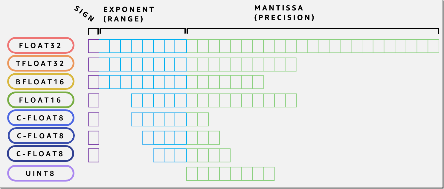
Typical data type bit representations.

In the context of LLM inference, floating point representations are commonly employed. Floating-point numbers follow the IEEE 754 standard and are represented using three components:

$$x = (-1)^{\text{sign}} \times (1 + \text{mantissa}) \times 2^{(\text{exponent} - \text{bias})}$$

where:

• Sign bit (1 bit): Determines if the number is positive (0) or negative (1)
• Exponent bits ($e$ bits): Encodes the power of 2, stored with a bias to allow both positive and negative exponents
• Mantissa bits ($m$ bits): Also called the significand or fraction, represents the precision of the number

Common floating-point formats include:

• FP32 (32 bits): 1 sign + 8 exponent + 23 mantissa, bias = 127, range ≈ $\pm 3.4 \times 10^{38}$
• FP16 (16 bits): 1 sign + 5 exponent + 10 mantissa, bias = 15, range ≈ $\pm 6.5 \times 10^{4}$
• BF16 (16 bits): 1 sign + 8 exponent + 7 mantissa, bias = 127, range ≈ $\pm 3.4 \times 10^{38}$
• FP8 E4M3 (8 bits): 1 sign + 4 exponent + 3 mantissa, bias = 7, range ≈ $\pm 448$
• FP8 E5M2 (8 bits): 1 sign + 5 exponent + 2 mantissa, bias = 15, range ≈ $\pm 5.7 \times 10^{4}$

The mantissa is stored in normalized form, where the leading bit is implicitly 1 (i.e., $1.\text{mantissa}$), except for subnormal numbers. Subnormal numbers (also called denormalized numbers) are very small values near zero that use a special encoding with an exponent of all zeros and an implicit leading bit of 0, allowing representation of values smaller than the smallest normal floating-point number. More exponent bits provide greater dynamic range, while more mantissa bits provide greater precision.

Let us see the floating point conversion in action; to illustrate quantization between floating-point formats, consider converting the value 6.625 from FP32 to FP8 E4M3 format.

FP32 representation (1 sign bit, 8 exponent bits, 23 mantissa bits):

• Binary representation: $6.625_{10} = 110.101_2$
• Normalized form: $1.10101_2 \times 2^2$
• Sign bit: $0$ (positive)
• Exponent: $2 + 127 = 129 = 10000001_2$ (bias of 127)
• Mantissa: $10101000000000000000000_2$ (23 bits, storing fractional part $.10101$)
• Full FP32: 0 10000001 10101000000000000000000

FP8 E4M3 representation (1 sign bit, 4 exponent bits, 3 mantissa bits):

• Sign bit: $0$ (positive)
• Exponent: $2 + 7 = 9 = 1001_2$ (bias of 7 for E4M3)
• Mantissa: Must round $.10101$ to 3 bits → $.101_2$ (round to nearest)
  • The 4th and 5th bits are $01$, which is less than half ($10$), so we round down
• Full FP8: 0 1001 101

Result: The FP8 E4M3 value represents $1.101_2 \times 2^2 = 1.625 \times 4 = 6.5$

Quantization error: $\epsilon = |6.625 - 6.5| = 0.125$

This example demonstrates how the limited mantissa precision in FP8 (3 bits vs. 23 bits) introduces quantization error. The representation is reduced from 32bits to 8bits, compressing the value by 4× but with precision loss.

Sources and impact of quantization error #

Quantization error arises from two fundamental limitations when mapping from a richer representation $S$ to a more constrained representation $T$: reduced dynamic range and reduced precision. Understanding these error sources is critical for successful model quantization, as uncontrolled quantization error can lead to catastrophic model failure or subtle performance degradation during inference.

Reduced dynamic range: overflow and underflow #

The dynamic range of a numerical format determines the span of values it can represent, from the smallest non-zero value to the largest finite value. When quantizing to a format with reduced dynamic range, values outside the representable range must be clipped, leading to overflow and underflow errors.

Overflow occurs when $|x| > \max(T)$, where the value exceeds the maximum representable value in the target format:

$$Q(x) = \max(T) \text{ if } x > \max(T), \text{ and } \min(T) \text{ if } x < \min(T)$$

For example, FP8 E4M3 has a maximum value of 448, while FP32 can represent values up to $\sim 3.4 \times 10^{38}$. A weight value of 500 in FP32 would be clipped to 448 in FP8 E4M3, causing saturation.

Underflow occurs when $0 < |x| < \min(|T|)$, where the value is smaller than the smallest representable non-zero value: $$Q(x) \approx 0$$

This is particularly problematic for activations with long-tail distributions, where small but important values are rounded to zero, effectively eliminating their contribution to subsequent computations.

Outliers and activation spikes: Neural network weights and activations often contain outliers—rare but large magnitude values. These outliers are especially problematic during inference quantization:

• If the quantization range is set to accommodate outliers, the majority of values are quantized with poor resolution
• If the range is set to capture the typical distribution, outliers saturate, potentially causing severe accuracy degradation

A single outlier channel in a transformer attention layer can dominate the quantization range, forcing all other channels to use a coarser quantization grid. Research has shown that just 0.1% of outlier features can account for significant quantization error in large language models, particularly in specific attention heads and feed-forward layers.

Reduced precision: rounding errors and numerical instability #

Even when values fall within the representable range, limited mantissa bits cause precision loss, where distinct values in $S$ map to the same value in $T$: $$Q(x_1) = Q(x_2) = x_q \text{ for } x_1 \neq x_2$$

This quantization-induced loss of information manifests in several ways during inference:

Accumulation of rounding errors: Each quantized operation introduces rounding error, and these errors accumulate as activations flow through the network. In transformer models with 32, 48, or more layers, even small per-layer errors can compound into significant output degradation.

Numerical instability in critical operations: Operations like normalization (LayerNorm, RMSNorm) and attention softmax are particularly sensitive to precision loss: $$\text{softmax}(x_i) = \frac{e^{x_i}}{\sum_j e^{x_j}}$$

When computed in low precision, the exponential function can amplify small quantization errors, and the normalization denominator may lose precision, leading to NaN or inf values. The attention mechanism’s dot-product can also overflow when sequence lengths are large, as it computes $QK^T$ where values can grow with $\sqrt{d_k}$.

Loss of discriminative ability: In classification or next-token prediction tasks, the model’s logits may lose the precision needed to distinguish between similar options. If the quantization step size is larger than the difference between competing logits, the model may produce incorrect predictions. This is especially problematic for language models where probability distributions over large vocabularies require fine-grained discrimination.

Impact on inference quality #

The cumulative effect of quantization error propagates through the network during inference, with deeper layers experiencing compounded errors. For large language models, this can manifest as:

• Perplexity degradation: Increased perplexity on language modeling tasks, indicating worse prediction quality and less confident probability distributions
• Task accuracy drop: Reduced performance on downstream tasks like question answering, summarization, classification, or reasoning
• Generation quality issues: Incoherent text, repetition, grammatical errors, factual inconsistencies, or hallucinations during text generation
• Complete failure modes: In extreme cases, the quantized model may produce garbage outputs, get stuck in loops, or encounter numerical errors (NaN/inf)

The severity of these issues depends on the target bit-width, the quantization scheme, and the model architecture.

Importance of controlling quantization error #

Effective quantization requires carefully managing the trade-off between compression and accuracy. Key strategies for inference quantization include:

1. Mixed-precision quantization: Using higher precision for sensitive layers (e.g., first/last layers, attention, layer norms) and lower precision for less sensitive components
2. Outlier management: Handling outliers through techniques like per-channel quantization, group quantization, or explicit outlier extraction and separate handling
3. Granularity selection: Choosing the appropriate level of quantization (per-tensor, per-channel, per-group) to balance accuracy and efficiency

The goal is not to eliminate quantization error (which is impossible) but to ensure it remains small enough that model behavior is preserved within acceptable tolerances. For LLM deployment, this typically means maintaining perplexity within 1-2% of the full-precision baseline while achieving 2-4× memory compression and computational speedup.

In the following sections, we will explore specific quantization schemes and techniques that address these challenges, enabling practical deployment of large language models.

Techniques to reduce quantization error #

Reducing model quantization errors to enable low precision deployment of LLMs is a very active research area.

Scaling for dynamic range adjustment Due to the smaller dynamic range of low precision data types the parameters are often scaled to fit in a particular range and then quantized afterwards. The granularity of this scaling is an important variable in determining the quantization error. Previous approaches have used tensor-wise, channel-wise scalings while more recently the granularity is further increased by decreasing the block size down to 16 or 32.

Tensor-wise and channel-wise scaling In the tensor-wise approach whole of a tensor is scaled to within the target range, whereas, for the channel-wise scaling the scaling would be along the output channel dimension. The less granular approaches are easier to implement and results in less memory overhead due to a smaller number of scales. However, the outliers would have a larger influence on the model; especially outlier within a group may result in underflow of small values in that particular block.

Micro-scaling formats Micro-scaling formats (MX) are proposed for a better control of outliers. These formats extend the concept of group-wise quantization by applying it at a very fine granularity with a standardized block structure. MX formats use individual scale factors for small blocks of elements (typically 16-32 elements):

$$x_q^{(i)} = Q\left(\frac{x^{(i)}}{s_{\lfloor i/B \rfloor}}\right)$$

where $B$ is the block size and $s_j$ is the shared scale factor for block $j$. The MX formats are supported in latest accelerators such as Blackwell GPUs and AWS Trainium 3.

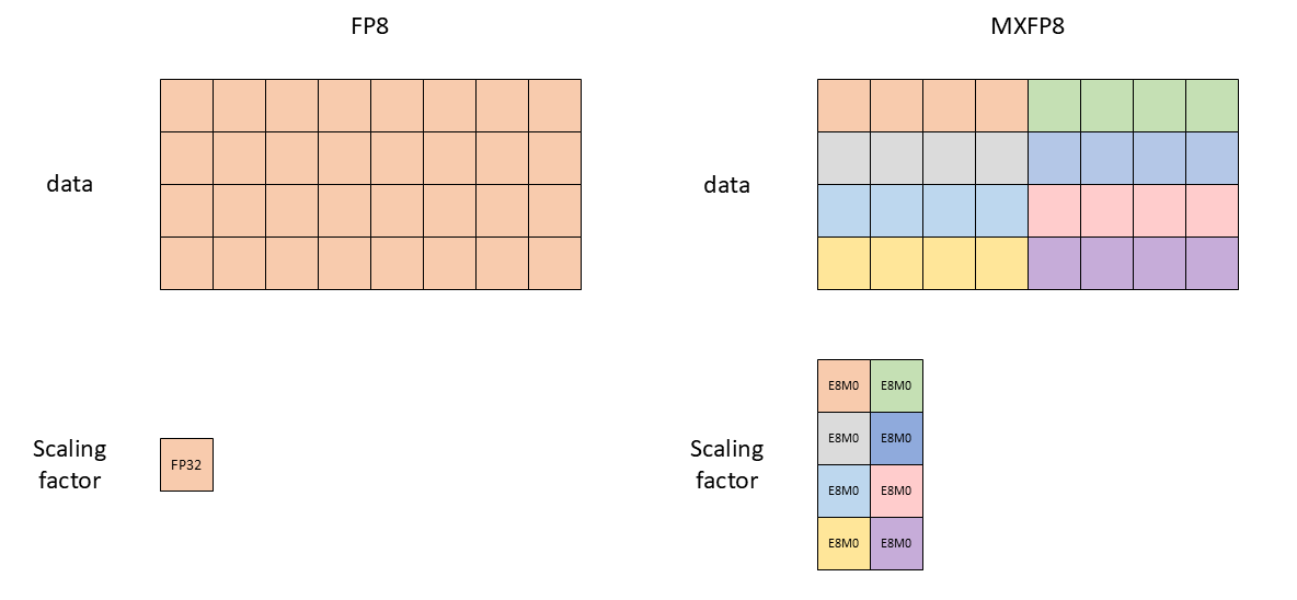
Tensor-wise vs MX format scaling factors (source docs.nvidia.com).

Random Hadamard transformation is a preprocessing technique that redistributes the dynamic range of tensors, making them more uniform and easier to quantize. The Hadamard matrix $H_n$ is an orthogonal matrix with entries $\pm 1$:

$$H_n H_n^T = n \cdot I_n$$

For a weight matrix $W$, the transformation applies:

$$W’ = D_1 H_d W H_d D_2$$

where $H_d$ is a Hadamard matrix and $D_1, D_2$ are random diagonal scaling matrices with entries $\pm 1$. Hadamard transforms are orthogonal and spread information uniformly. A single outlier value gets distributed across multiple positions, reducing peak magnitudes. The transformation makes the distribution of values more uniform, better utilizing the quantization codebook. Can be efficiently computed in using the Fast Walsh-Hadamard Transform. By applying the same rotation to inputs and outputs of adjacent layers, the rotations can be absorbed into the weight matrices without changing the model’s mathematical function.

How to quantize a model? #

There are several ways of converting a high precision model to lower precisions. These approaches differ in when quantization is applied, whether calibration data is required, and what computational resources are needed.

Post-training quantization is the most common approach for inference optimization, where a pre-trained full-precision model is quantized without any additional training or fine-tuning. PTQ is attractive because it requires no access to the original training data or training pipeline and is computationally inexpensive. To mitigate the accuracy loss, the PTQ process may involve a pass through a small calibration dataset to fine-tune the model for quantization. PTQ may include advanced methods like SpinQuant, Quip, GPTQ that optimize quantization parameters or apply layer-wise fine-tuning to minimize error. The PTQ methods often employ advanced techniques such as RHT to control the quantization error.

One-shot quantization can be seen as a subset of PTQ that quantizes the model without requiring any calibration data. It relies solely on the weight statistics themselves to determine quantization parameters. This approach enables immediate quantization of any model without data collection, is useful when calibration data is unavailable or privacy-sensitive, may perform poorly for aggressive quantization (4-bit or lower) or activation quantization. One-shot methods are commonly used for quick deployment scenarios where a small accuracy drop is acceptable in exchange for maximum simplicity. They serve as a baseline for more sophisticated PTQ approaches.

Quantization-aware training simulates quantization during the training or fine-tuning process, allowing the model to adapt to quantization constraints. During forward passes, weights and activations are quantized, but gradients are computed using straight-through estimators (STE) or other function approximations to enable backpropagation. QAT typically achieves the best accuracy, especially for aggressive quantization (4-bit or lower), but has significant drawbacks for LLM deployment:

• Computational cost: Requires full model training or fine-tuning, which can take days or weeks on large clusters
• Data requirements: Needs access to large-scale training data, which may be unavailable or proprietary
• Flexibility: Less flexible for exploring different quantization configurations post-deployment

For these reasons, QAT is less commonly used in LLM inference scenarios, where PTQ methods have proven surprisingly effective. However, QAT remains valuable when maximum accuracy at very low bit-widths is critical, or when quantization is planned from the start of model development.

Note: While this tutorial focuses on inference, understanding QAT is valuable as some publicly released models may have been prepared using QAT techniques.

Performance benefits (storage and speedup) #

Quantization provides two primary performance benefits for LLM deployment: reduced memory footprint and increased inference throughput. Reduced memory footprint is straight-forward due to the lower bit representations used. Increased inference throughput depends on hardware support.

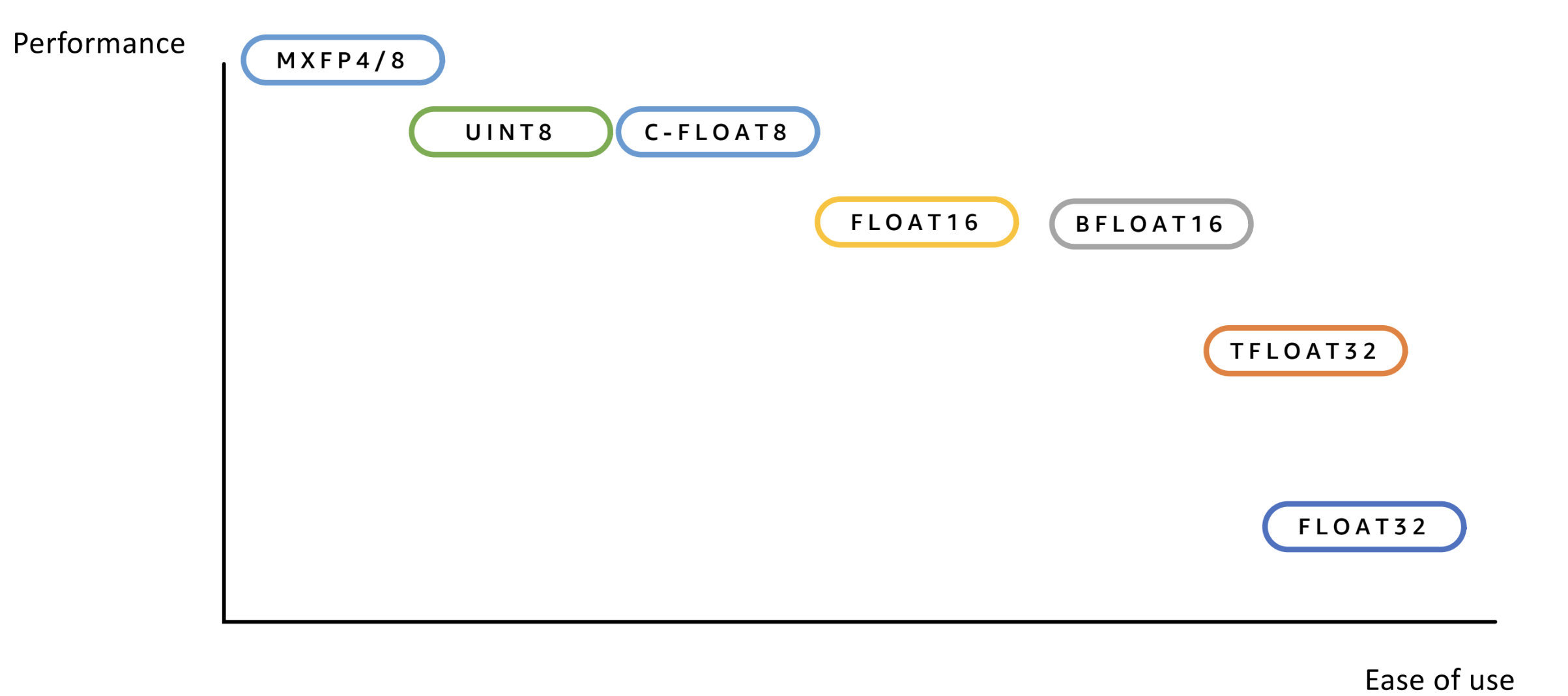
Performance vs. ease of use of different data types.

• Weight-only quantization: Only model weights are quantized, while activations remain in higher precision (FP16/BF16). This reduces memory footprint and bandwidth, as quantized weights require less storage. However, during computation, weights must be dequantized back to high precision to perform the actual matrix multiplications, which limits computational speedup. The primary benefit is memory savings rather than compute acceleration.
• Weight-activation quantization: Both weights and activations are quantized, enabling greater speedup because low-precision matrix multiplications (matmuls) can be executed directly on supported hardware, which is significantly faster than high-precision operations. This approach requires more careful calibration to maintain accuracy, as both weights and activations contribute to quantization error.
• KV cache quantization: The key-value cache used during autoregressive decoding can also be quantized to reduce memory footprint, which is particularly important for long-context scenarios. This is discussed in more detail later in the KV cache compression section.

Matrix multiplication (Matmul): Backbone of LLM computation #

The speed of inference is often determined by the speed of matrix multiply operations. Recent hardware support matrix multiplications of as low as 4 bit floating point representations. Low precision matrix-multiply accumulate (MMA) operations on (supported) hardware are generally faster compared to high precision ones due to occupying less space on the hardware (i.e. given a fixed area of the chip one can fit more low-precision matmul circuitry). For instance, an FP4 matmul is approximately twice as fast than an FP8 matmul, which is in turn twice as fast as a BF16 matmul on the supported Nvidia chips (e.g. Blackwell).

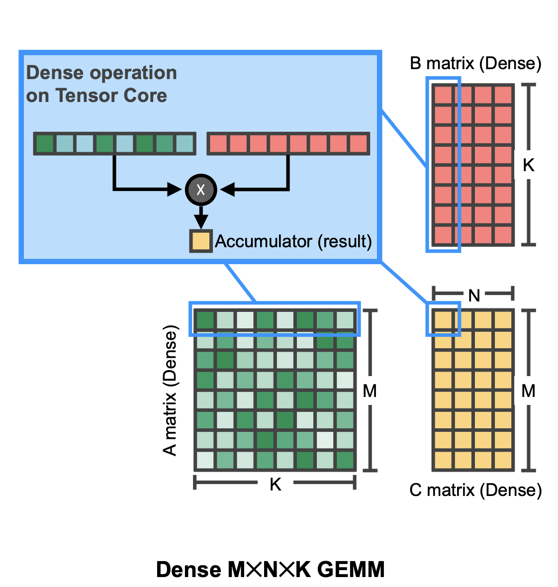
Dense matmul visualization (Mishra et al.).

Different hardware providers use different approaches for MMA. In particular, Nvidia uses flexible tensor cores, whereas, Google TPUs and AWS Trainium use less flexible but high utility systolic arrays.

Not all matmuls are equal #

Moden LLM architectures are based on transformers that include many different components. Some of these components are more sensitive to low precision operations, these include matmuls in core attention (QK, PV), softmax, input-output embedding. In contrast, MLP layers seem to be relatively robust to quantization while also dominating the FLOP for common sequence length selections.

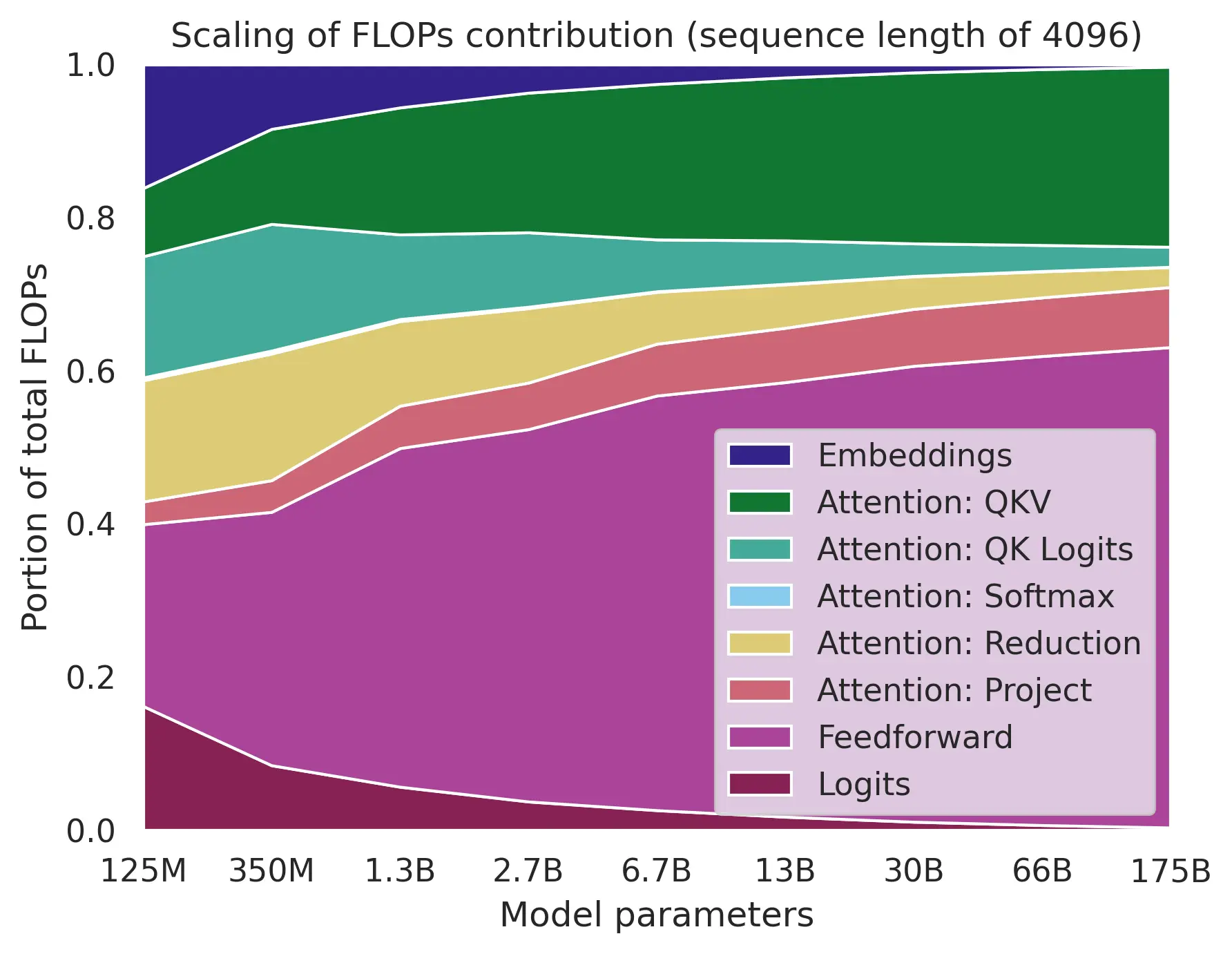
Flop distribution across different operations (source: adamcasson.com).

However, during inference the sequence length may become so large that FLOP can start to be dominated by the core attention matmuls.

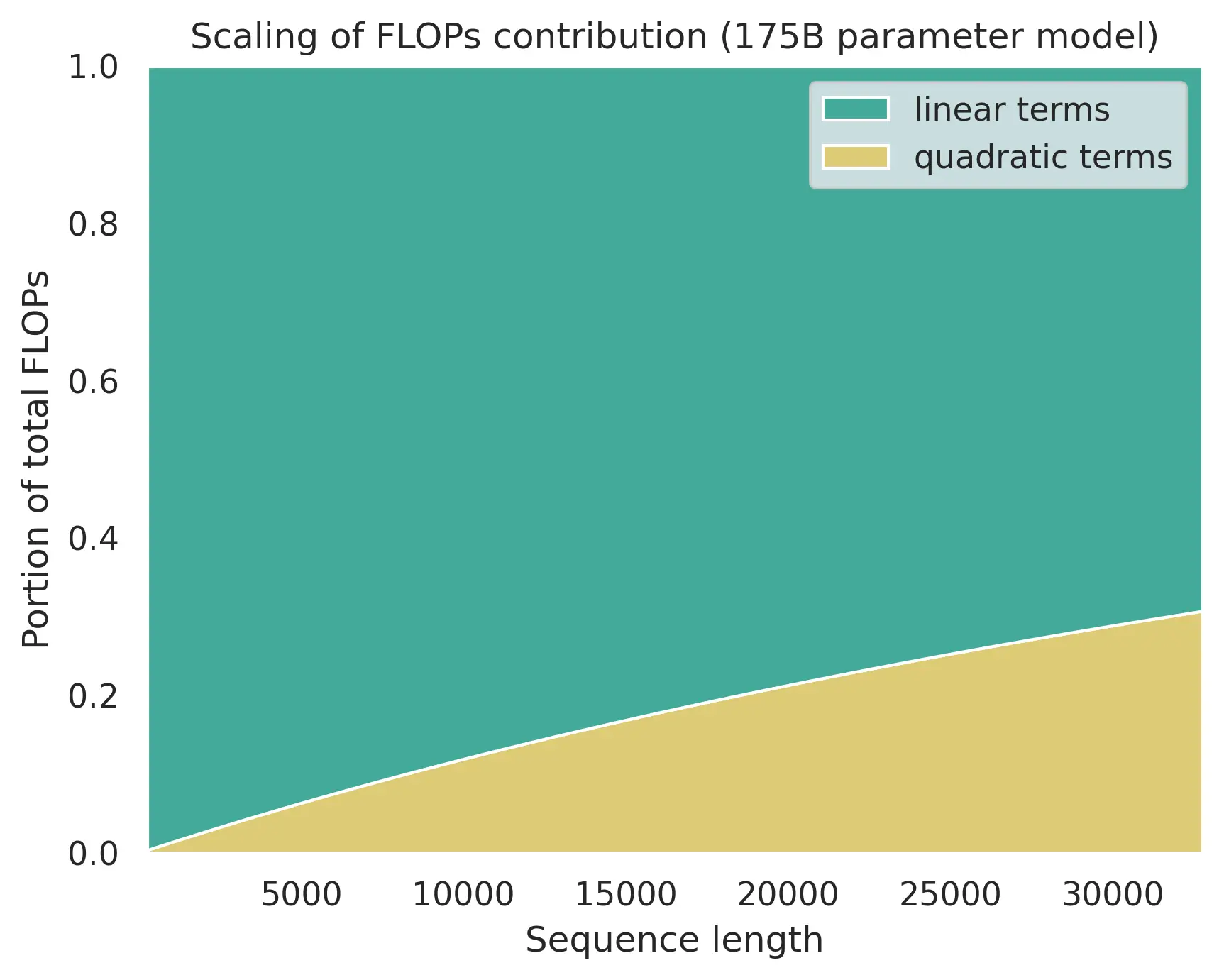
Flop distribution with increased sequence length (source: adamcasson.com).

Recently, quantizing the attention gained more attention, resulting in works that try to use 4/8-bit precision for core attention. This works include FlashAttention3, SageAttention3 and so on. This is an important future direction for model quantization research.

References #

1. Mishra, Asit, et al. “Accelerating sparse deep neural networks.” arXiv preprint arXiv:2104.08378 (2021).
2. Zhang, Jintao, et al. “Sageattention3: Microscaling fp4 attention for inference and an exploration of 8-bit training.” arXiv preprint arXiv:2505.11594 (2025).
3. Shah, Jay, et al. “Flashattention-3: Fast and accurate attention with asynchrony and low-precision.” Advances in Neural Information Processing Systems 37 (2024): 68658-68685.
4. Casson, Adam. “Transformer FLOPs.” https://www.adamcasson.com/posts/transformer-flops