Efficient Attention Variants #

At the heart of the success of transformer architectures, lies the attention mechanism, which allows models to capture long-range dependencies and complex interactions across inputs. However, standard self-atention scales quadratically with sequence length, making it prohibitively expensive for large-scale or realtime applications. This has spurred a wave of research into efficient attention mechanisms – techniques that reduce the computational and memory overhead without sacrificing accuracy. Some of them are highlighted here.

Multi Head Attention (MHA) #

MHA is a core optimization, in which instead of computing a single attention distribution over the input sequence, the model’s hidden dimension is split into multiple heads. Each head learns its own set of query, key, and value projection, and the model computes scaled dot-product attention independently for each head, resulting in multiple attenton outputs. These outputs are then concatenated and linearly projected back to the model’s original dimension.

Suppose the input to the attention layer is a sequence of hidden states,

$$X \in \mathbb{R}^{T \times d_{\text{model}}},$$

where $T$ is the sequence length, and $d_{\text{model}}$ is the embedding dimension. For each head $h \in {1, \ldots, H}$ (where $H$ is the number of attention heads), we compute separate query, key, and value matrices via learned linear projections:

$$Q_h = XW_h^Q, \hspace{3ex} K_h = XW_h^K, \hspace{2ex} V_h = XW_h^V$$

where $W_h^Q, W_h^K, W_h^V \in \mathbb{R}^{d_{\text{model}} \times d_k}$. Here, $d_k = d_{\text{model}}/H$ is the dimension per head.

Each head performs scaled dot-product attention:

$$O_h \triangleq \text{Attention}(Q_h, K_h, V_h) = \text{softmax}\left(\frac{Q_hK_h^\top}{\sqrt{d_k}}\right)V_h \in \mathbb{R}^{T \times d_k}.$$

The outputs from all heads are concatenated to get:

$$O = \text{Concat}(O_1, O_2, \ldots, O_H) \in \mathbb{R}^{T \times d_{\text{model}}}$$

A final linear projection matrix $W^O \in \mathbb{R}^{d_{\text{model}} \times d_{\text{model}}}$ yields the final output:

$$\text{MHA}(X) = OW^O$$

This parallel attention structure has two key benefits:

1. It increases the models’ representation capacity without increasing computational complexity as much as a single very large attention would,
2. It allows the model to capture richer contextual information because different heads can specialize in attenting to different positions or patterns in the sequence. For example, one head might learn to track subject-verb agreement, while another focuses on long-range dependencies.

The final output provides a more expressive representation that downstream layers can use effectively. MHA (along with GQA, which is described next) is visualized below.

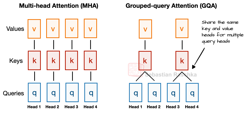
Comparison of Multi Head Attention (MHA) vs Grouped Query Attention (GQA) (credits: Sebastian Raschka)

Grouped Query Attention (GQA) #

Where standard MHA has one set of key/value projections per query head, GQA [3] reduces the number of key/value heads to save memory and bandwidth during inference, while keeping the same number of query heads for expressivity. Let $G$ be the total number of key/value heads (with $G < H$, i.e., the number of query heads). Denote by $d_q = d_{\text{model}}/ H$ and $d_{kv} = d_q$ be the dimension per query head and per KV head, respectively.

For each head $h = 1, \ldots, H$, the query is given by $Q_h = XW_h^Q$, where $W_h^Q \in \mathbb{R}^{d_{\text{model}} \times d_q}$.

For keys and values (fewer heads), for $g = 1, \ldots G$ and $W_g^K, W_g^V \in \mathbb{R}^{d_{\text{model}} \times d_{kv}}$, we have,

$$K_g = XW_g^K \hspace{2ex} \text{and} \hspace{2ex} V_g = XW_g^V.$$

Each query head $h$ is assigned to one key/value head $g$. For example, if $r = H/G$ (an integer), then $g = \left\lfloor \frac{h}{r} \right\rfloor$. This means $r$ query heads share the same key/value pair. Subsequently, for each query head $h$, we attend to the key/value head $g$ it’s mapped to, to get:

$$O_h \triangleq \text{Attention}(Q_h, K_g, V_g) = \text{softmax}\left(\frac{Q_hK_g^\top}{\sqrt{d_q}}\right)V_g \in \mathbb{R}^{T \times d_q}.$$

As in standard MHA,

$$\text{GQA}(X) = OW^O, \hspace{2ex} W^O \in \mathbb{R}^{d_{\text{model}} \times d_{\text{model}}}, \hspace{2ex} O = \text{Concat}(O_1, O_2, \ldots, O_H) \in \mathbb{R}^{T \times d_{\text{model}}}.$$

With GQA, the KV cache size is given by,

$$\text{batchsize } * \text{ seqlen } * \text{ (embed-dim / nheads) } * \text{ nlayers } * \hspace{1px} 2 \hspace{1px} * \text{ precision } * \text{ nKVheads }$$

GQA offers a balance between efficiency and expressivity in transformer architectures. By allowing many query heads to share a smaller number of KV heads, GQA drastically reduce the memory footprint and bandwidth cost of KV caching during autoregressive inference – often by a factor of $H/G$, where $H$ is the number of query heads and $G$ is the number of KV heads. This reduction leads to faster decoding, lower latency, and better scalability to longer context lengths. In practice, this enables deploying larger or more capable models under the same memory budget, making GQA a key ingredient in efficient long-context language models like Llama 2 [4] and Llama 3 [5].

Multi-Head Latent Attention (MLA) #

As an alternative to GQA, DeepSeek V3/R1 introduced MLA, in which instead of sharing key and value heads like GQA, MLA compresses the key and value tensors into a lower-dimensional space before storing them in the KV cache. At inference, compressed tensors are re-expanded to their original dimensions, trading an extra matrix multiplication for reduced memory footprint, since only the latent states are cached. More specifically, for each token:

$$Z_t = X_t W_Z,\quad W_Z \in \mathbb{R}^{d \times d_\ell},\quad d_\ell \ll d.$$

Instead of caching $K_t, V_t \in \mathbb{R}^d$, we cache the latent vector $Z_t \in \mathbb{R}^{d_\ell}$ once per token. The core of MLA is this low-rank joint compression for attention keys and values to reduce Key-Value (KV) cache during inference. Each attention head $h$ has its own projections from the latent space:

$$K_t^{(h)} = Z_t W_K^{(h)},\quad V_t^{(h)} = Z_t W_V^{(h)}$$

Queries are still head-specific, i.e., $Q_t^{(h)} = X_t W_Q^{(h)}$. Once the keys and values are reconstructed, attention is computed as before. Since $d_\ell \ll d$, this results in a massive reduction in KV cache memory footprint, which is excellent for long-context decoding. As with GQA, this is orthogonal to other KV cache compression techniques like quantization. Moreover, the DeepSeek V2 [7] paper showed some ablation studies that MLA outperforms MHA with MoE architectures. The only downside of MLA is the added computation due to the extra projection FLOPs involved in obtaining $K^{(h)}, V^{(h)}$ from $Z$, but this is not a major concern because autoregressive decoding is memory-bandwidth bound. MLA is visualized below.

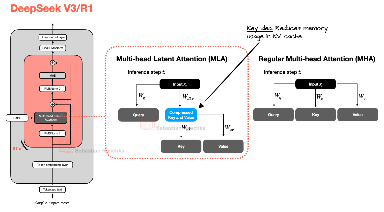
Comparison between MLA (used in DeepSeek V3 and R1) and regular MHA (credits: Sebastian Raschka)

Sliding Window Attention (SWA) #

In standard full attention, each token attend to every other token in the sequence. This results in quadratic complexity, i.e., $\mathrm{O}(N^2)$, where $N$ is the sequence length. Sliding window Attention (SWA) changes this by restricting the attention span. In SWA, each token only attends to tokens within a fixed window of size $w$ around it (e.g., for casual SWA, this corresponds to the previous $w$ tokens). This reduces the computational complexity to $\mathrm{O}(Nw)$, instead of $\mathrm{O}(N^2)$, which is particularly useful for long contexts such as long documents or streaming scenarios, without blowing up GPU memory. With SWA, the KV cache size is given by,

$$\text{batchsize } * \text{ W } * \text{ (embed-dim / nheads) } * \text{ nlayers } * \hspace{1px} 2 \hspace{1px} * \text{ precision } * \text{ nKVheads. }$$

That is, SWA reduces the KV cache size by a factor of $\text{W / seqlen}$

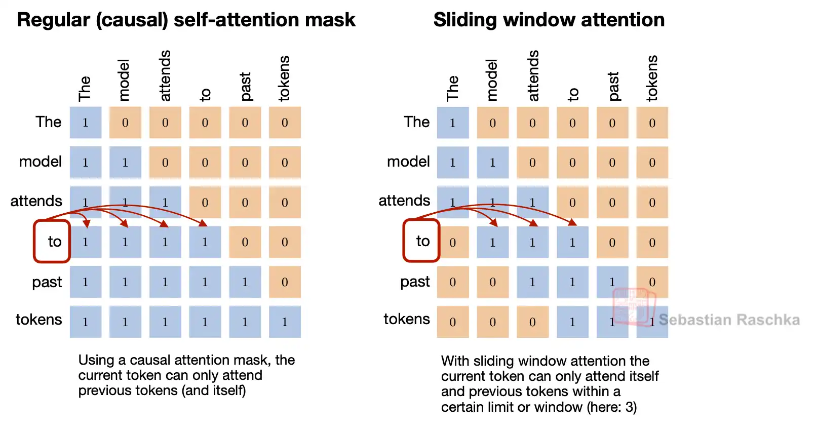
Comparison of standard attention vs sliding window attention (credits: Sebastian Raschka)

Sparse Attention #

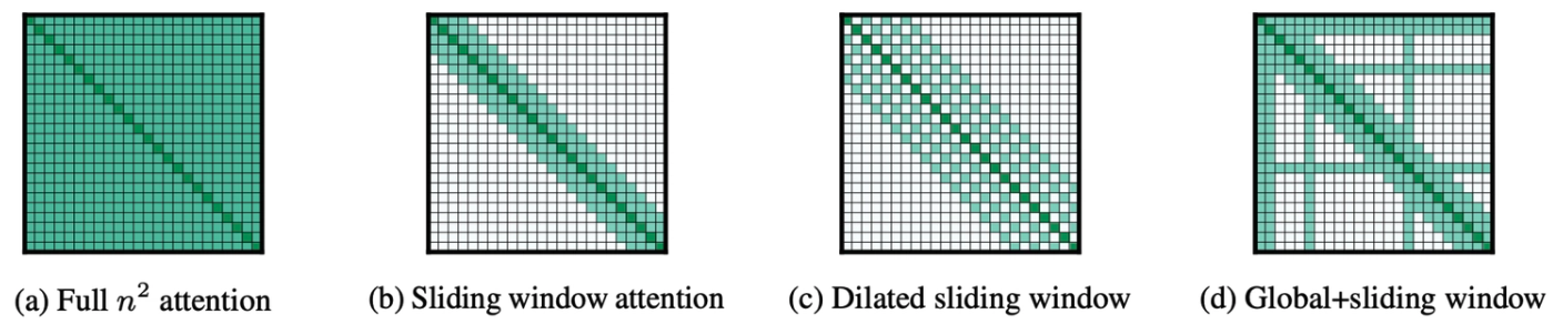
Sparse attention generalizes the SWA by relaxing the constraint of sliding window and allowing attention to be computed over arbitrary subsets of token pairs, as long as the pattern is structured or constrained. From this perspective, SWA corresponds to a particular sparsity pattern—one that is local, uniform, and easy to implement—while sparse attention encompasses a broader family of patterns that selectively introduce non-local interactions. Generally, sparse attention restricts which token pairs can attend to each other, reducing the effective attention matrix size while preserving task-relevant context. From an inference perspective, sparse attention is attractive because it:

• Reduces FLOPs and memory bandwidth
• Lowers KV-cache growth for long contexts
• Enables better cache locality and kernel fusion opportunities
• Makes long-context inference feasible on fixed hardware budgets

At inference time, this generalization enables a richer tradeoff between expressivity and efficiency. By activating only a subset of attention links, such as combining local windows with strided, global, or block-structured connections, sparse attention reduces the quadratic cost of dense attention while preserving important long-range dependencies. However, unlike SWA, which maps cleanly to regular kernels and predictable memory access, general sparse patterns introduce additional systems challenges, including irregular memory access, and kernel specialization. As a result, sparse attention shifts the optimization focus from algorithmic complexity alone to hardware and runtime-aware execution, making it a nontrivial tool for scalable long-context inference.

Sparse Attention Mechanisms selectively attend to specific past tokens (credits: klu.ai/glossary)

A number of influential papers have explored such mechanisms in practice. For example, Longformer [8] introduces a hybrid sparse pattern combining local windows with a small number of global tokens to preserve important long-range context while keeping computation linear in sequence length. BigBird [9] proposes block-sparse attention with local, random, and global components to approximate full attention with linear complexity. We do not exhaustively cover the different sparse attention mechanisms.

References #

1. Sliding Window Attention (SWA) https://sebastianraschka.com/llms-from-scratch/ch04/06_swa/

2. The big LLM architecture comparison https://magazine.sebastianraschka.com/p/the-big-llm-architecture-comparison

3. GQA: Training Generalized Multi-Query Transformer Models from Multi-Head Checkpoints https://arxiv.org/abs/2305.13245

4. Llama 2: Open Foundation and Fine-Tuned Chat Models https://arxiv.org/abs/2307.09288

5. The Llama 3 Herd of Models https://arxiv.org/abs/2407.21783

6. DeepSeek-V3 Technical Report https://arxiv.org/abs/2412.19437

7. DeepSeek-V2: A Strong, Economical, and Efficient Mixture-of-Experts Language Model https://arxiv.org/abs/2405.04434

8. Longformer: The Long-Document Transformer, Beltagy et. al., 2020 https://arxiv.org/abs/2004.05150

9. Big Bird: Transformers for Longer Sequences, Zaheer et; al., 2021 https://arxiv.org/abs/2007.14062