Speculative Decoding #
By default, LLM decoding generates one token at a time. During each decoding step, the model loads the KV cache of all previous tokens but only computes attention for a single new token. This process is memory-bound and under-utilizes the available compute resources, as modern accelerators are designed for parallel processing of multiple tokens (as seen in the prefill phase).
Speculative Decoding (SD) is a technique that improves the throughput of token generation by breaking the sequential bottleneck. The key insight is to use a lightweight drafter model to predict multiple future tokens, then have the main target model verify these predictions in parallel. This transforms the memory-bound sequential decoding into a compute-bound parallel verification process, similar to prefill.
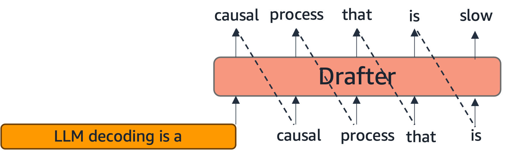
In speculative decoding, the target model (the main LLM) is paired with a lightweight drafter, which could be another much smaller LLM or a specialized model derived from the target. The drafter predicts multiple tokens into the future (illustrated left below), and the target model verifies these tokens in parallel (illustration right below).
The Verification Process #
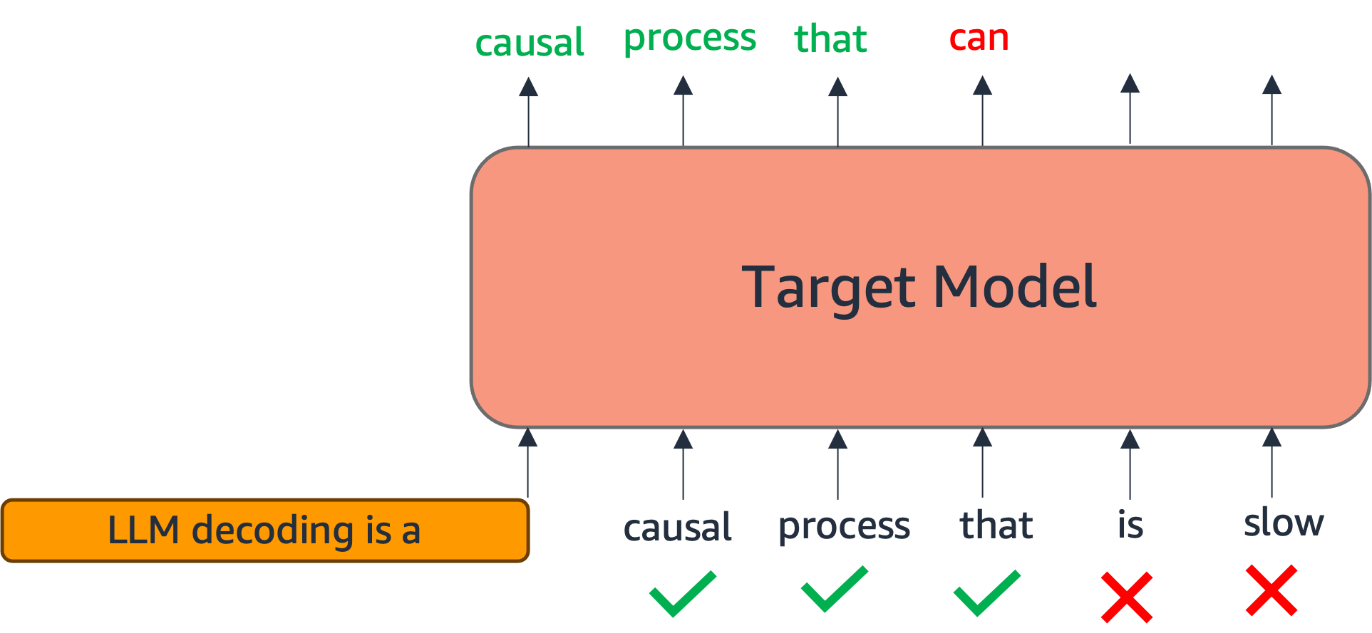
The verification step inputs the prompt and the drafter’s generation together to the target model. The prompt’s KV cache is loaded, and attention is computed for multiple drafted tokens all at once. This is similar to prefilling and better utilizes compute resources by processing multiple tokens in parallel.
Formally, if the drafter generates a sequence of $\gamma$ tokens $(t_1, t_2, \ldots, t_\gamma)$, the target model processes the concatenated sequence $[\text{prompt}; t_1, t_2, \ldots, t_\gamma]$ in a single forward pass. For each position $i \in {1, 2, \ldots, \gamma}$, the target model computes the probability distribution $p_{\text{target}}(\cdot | \text{prompt}, t_1, \ldots, t_{i-1})$ over the vocabulary.
Acceptance and Rejection Mechanism #
The verification process uses an acceptance criterion to determine which drafted tokens to keep. For each drafted token $t_i$ at position $i$, we compare the target model’s probability $p_{\text{target}}(t_i | \text{prompt}, t_1, \ldots, t_{i-1})$ with the drafter’s probability $p_{\text{drafter}}(t_i | \text{prompt}, t_1, \ldots, t_{i-1})$. A common acceptance criterion is:
$$\text{accept } t_i \text{ if } \frac{p_{\text{target}}(t_i)}{p_{\text{drafter}}(t_i)} \geq r$$
where $r$ is a threshold. This ensures that the distribution of accepted tokens matches the target model’s distribution, maintaining correctness.
The first token that fails the acceptance criterion triggers rejection. All subsequent tokens are discarded, and we fall back to the target model’s generation starting from that position. The best case occurs when all $\gamma$ drafted tokens are accepted, providing maximum speedup. The worst case occurs when the first drafted token fails to match, but even then, we simply use the first token generated by the target model, falling back to standard decoding behavior.
Crucially, speculative decoding is lossless: The output distribution is identical to that of conventional decoding using only the target model. This is guaranteed by the acceptance mechanism, which ensures that only tokens that would have been generated by the target model are accepted.
Speedup Analysis #
The speedup from speculative decoding depends on two key factors:
-
Acceptance rate: How many drafted tokens are accepted on average. If $\alpha$ tokens are accepted on average from $\gamma$ drafted tokens, the effective tokens generated per target model forward pass is $1 + \alpha$ (an one additional token is generated by the target model).
-
Drafter speed: How much faster the drafter is compared to the target model. If the drafter is $k$ times faster, and we draft $\gamma$ tokens, the total time is approximately:
$$\text{SDTime} = \text{DrafterTime}(\gamma) + \text{TargetTime}(1 + \alpha)$$
Compared to standard decoding which requires $\text{TargetTime}(1 + \alpha)$ sequential forward passes, the speedup is: $$\text{Speedup} = \frac{1 + \alpha}{1 + \frac{\text{DrafterTime}(\gamma)}{\text{TargetTime}(1 + \alpha)}}$$
A good drafter should be both fast (small $\text{DrafterTime}$) and accurate (high $\alpha$), generating continuations that closely match the target model’s distribution.
Eagle Drafter #
One approach to creating a drafter is to train a separate smaller model from scratch such that its generations match the target model’s (e.g., DistillSpec). However, training such a separate drafter requires significant computational overhead and may not fully leverage the target model’s learned representations.
Eagle (Li et al., 2024) is a state-of-the-art method that reuses intermediate hidden states and parameters of the target model, dramatically reducing training overhead while achieving high acceptance rates. The key innovation is to leverage the target model’s internal representations rather than training a completely independent drafter.
Architecture #
The Eagle drafter architecture is illustrated below, with the target model on the left and the drafter on the right. The drafter reuses two key components from the target model:
- Embedding layer: The same token embeddings used by the target model
- Language model head: The same output projection layer that maps hidden states to vocabulary logits
Additionally, the drafter extracts intermediate features $f_i$ from the target model’s hidden states (typically from an intermediate layer). The drafter then combines:
- Input token embeddings $e_i$ (from the shared embedding layer)
- Target model features $f_i$ (extracted from intermediate layers)
These are processed through a lightweight transformer decoder layer, which is the only trainable parameter in the drafter. This design makes the drafter extremely efficient while maintaining strong alignment with the target model’s behavior.
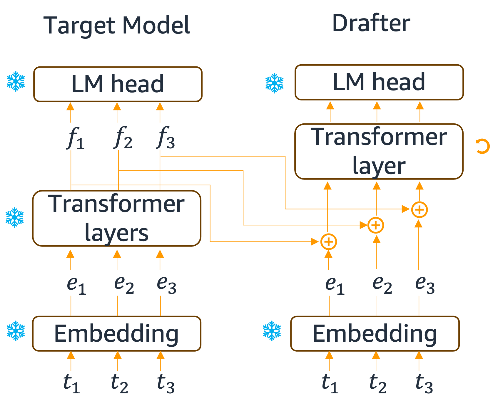
Eagle drafter architecture: reusing target model components (embedding, LM head) and intermediate features.
Training #
The drafter is trained to generate continuations that match the target model’s distribution. A simple approach is to generate continuations using the target model and use these as training data, then train the drafter by minimizing the next-token prediction loss on this dataset.
Another option is to use a more sophisticated distillation-based loss that minimizes the KL divergence between the drafter’s and target model’s logit distributions:
$$\mathcal{L} = \text{KL}(p_{\text{target}} || p_{\text{drafter}}) + \lambda \cdot \mathcal{L}_{\text{CE}}$$
where $\mathcal{L}_{\text{CE}}$ is the cross-entropy loss on target model generations, and $\lambda$ is a weighting factor. This approach ensures the drafter learns not just to predict the most likely tokens, but to match the entire probability distribution of the target model, leading to higher acceptance rates during verification.
Tree-structured Draft #
As an orthogonal approach to improve acceptance rates, one can draft multiple continuations simultaneously. This strategy increases the probability that at least one continuation will have high acceptance, while also better utilizing available compute resources.
Token Tree Structure #
Multiple draft continuations naturally form a tree structure because they often share common prefixes. For example, if we draft three continuations:
- Path 1: “The cat sat on the”
- Path 2: “The cat sat on a”
- Path 3: “The dog ran”
These form a tree where “The cat sat on” is a shared prefix, branching into “the” and “a”, while “The dog ran” forms a separate branch. This tree structure is efficient because shared prefixes only need to be computed once.
Practical Considerations and Limitations #
When Speculative Decoding is Most Beneficial #
Speculative decoding provides the greatest speedup when:
- High acceptance rates: The drafter generates continuations that closely match the target model
- Fast drafter: The drafter is significantly faster than the target model (typically 3-10×)
- Memory-bound regime: The system has available compute capacity that would otherwise be idle
- Long sequences: The benefits accumulate over many tokens, making the overhead worthwhile
The technique is less beneficial when:
- Low acceptance rates: If the drafter frequently fails, the overhead may outweigh benefits
- Compute-bound regime: If already compute-limited, additional parallelism may not help
- Short sequences: The overhead of drafting and verification may not be amortized
Trade-offs #
While speculative decoding can provide 2-3× speedup in practice, it comes with trade-offs:
- Memory overhead: Storing multiple draft tokens and their KV caches increases memory usage
- Complexity: The verification and acceptance logic adds system complexity
- Drafter training: Creating an effective drafter requires additional training or fine-tuning effort
- Variable latency: Acceptance rates vary, leading to variable per-token latency (though average throughput improves)
Integration with Other Optimizations #
Speculative decoding is complementary to other inference optimizations:
- KV cache quantization: Can be applied to both target and drafter models to reduce memory
- Continuous batching: Works well with dynamic batching systems
- Model parallelism: Can be applied across both target and drafter models
References #
-
Fast Inference from Transformers via Speculative Decoding, Leviathan et al., 2023 https://arxiv.org/abs/2211.17192
-
DistillSpec: Improving Speculative Decoding via Knowledge Distillation, Zhou et al., 2024 https://arxiv.org/abs/2310.08461
-
EAGLE: Speculative Sampling Requires Rethinking Feature Uncertainty, Li et al., 2024 https://arxiv.org/abs/2401.15077