Key-Value (KV) Caching #

A key optimization for accelerating autoregressive inference in large language models is Key–Value (KV) caching. Transformer-based LLM inference happens in two stages: prefill phase, when the prompt is processed, and decoding phase, when tokens are generated one-by-one. During prefill, each transformer layer computes attention keys K and values V for every input token. Without caching, the model would need to recompute the entire attention stack from scratch at every decoding step—an operation whose cost scales quadratically with the sequence length and quickly prohibits real-time inference. KV caching avoids this waste by storing the computed K and V tensors in memory, so that during decoding, the model only needs to compute attention for new tokens and can reuse the cached representations for all past tokens, avoiding redundant computations. The result is a drastic improvement in per-token latency and a shift in the performance bottleneck from compute to memory bandwidth. More specifically, the quadratic scaling of the attention layer is transformed into a linear scaling at the cost of increased memory utilization.

Causal attention enables computation reuse #

Consider a transformer decoder-only model with $L$ layers, $H$ attention heads, head dimension $d$, and hidden dimension $D = H \cdot d$. For a token sequence $(x_1, \ldots, x_T)$, denote the hidden representation entering layer $\ell$ at index $t$ by $h_t^{(\ell)} \in \mathbb{R}^D$. Each layer $\ell$ computes: $$Q^\ell_t = W^\ell_Q h^\ell_t, \qquad K^\ell_t = W^\ell_K h^\ell_t, \qquad V^\ell_t = W^\ell_V h^\ell_t,$$ where $W^\ell_Q, W^\ell_K, W^\ell_V \in \mathbb{R}^{D \times D}$. During prefill, this computation is done for all $t \in {1, \ldots, T}$.

For every layer $\ell$, the cache stores all the past keys and values as:

$$K^\ell_{\le t} = (K^\ell_1, \dots, K^\ell_t) \in \mathbb{R}^{t \times D}$$

$$V^\ell_{\le t} = (V^\ell_1, \dots, V^\ell_t) \in \mathbb{R}^{t \times D}.$$

These are appended once during prefill, then incrementally during decoding. This KV cache built during prefill, is re-used repeatedly during decoding as follows. Because of the causal mask, each token’s output depends only on representation from previous tokens. Since those earlier representations do not change across decoding steps, the output for a previously generated token remains the same at every iteration, making the repeated computation redundant.

As a concrete example, consider the sentence, The quick brown fox as the input sequence. For simplicity, assume each of these words correspond to a single token. Then the representations for the tokens, The, quick, brown, fox are computed during prefill, populating the KV cache. Suppose we generate the next token to be jumps as a continuation of the prompt The quick brown fox. Output representation of the last token, fox, depends only on the tokens up until that point, i.e., The quick brown fox, so its output representation would not change when the new token jumps is taken into consideration – enabling reuse of the past representations.

During the decoding phase, for a new decoding step at token index $t+1$, we compute $$Q^\ell_{t+1} = W^\ell_Q h^\ell_{t+1}, \qquad K^\ell_{t+1} = W^\ell_K h^\ell_{t+1}, \qquad V^\ell_{t+1} = W^\ell_V h^\ell_{t+1},$$ The attention scores for $h^\ell_{t+1}$ with respect to any previous token $i$, denoted as $\alpha_{t+1 ,i}$, is computed as follows: $$\alpha^\ell_{t+1, i} = \frac{\text{exp}\left(\frac{(Q^\ell_{t+1})^\top K^\ell_i}{\sqrt{d}}\right)}{\sum_{j=1}^{t+1}\text{exp}\left(\frac{(Q^\ell_{t+1})^\top K^\ell_j}{\sqrt{d}}\right)}$$ Note that the above computation reuses the cached $K^\ell_{\le t}$ for $i \leq k$. The contextualized output is computed by reusing $V^\ell_{\le t}$ as: $$z_{t+1}^\ell = \sum_{i=1}^{t+1}\alpha_{t+1,i}^\ell V_i^\ell$$ Crucially, the model does not recompute $K_i$ or $V_i$ for $i \leq t$; it loads them directly from the KV cache.

This (visualized below) is repeated for every subsequent auto-regressively decoded token, and the representations are appended to the KV cache (which keeps growing with the sequence length).

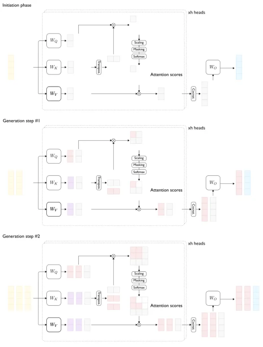
Every decoding step caches and reuses previously computed keys and values (red). Only blue blocks are new (credits: Pierre Lienhart)

Computation complexity with and without KV cache #

In the absence of KV cache, at each decoding step, attention is recomputed over all previous tokens. Hence, for a sequence length of $t$, we have, $$\text{Cost (without KV cache)} = \sum_{u=1}^{t+1}\text{O}(uD) = \text{O}(t^2D)$$

However, with KV cache, at time $t+1$, for each layer $\ell$, we need to query $Q_{t+1}^\ell$ , key $K_{t+1}^\ell$, and value $V_{t+1}^\ell$ only for the last token $t+1$, i.e., a compute cost of $\text{O}(D^2)$. Additionally, we need to do another single attention matvec with $K_{\le t}^\ell$, which incurs a cost of $\text{O}(tD)$. Therefore, $$\text{Cost (with KV cache)} = \text{O}(tD + D^2).$$ This reduces the quadratic growth with repect to $t$ to linear at the price of additional memory.

Memory footprint of KV cache #

For an LLM with $L$ layers, for each layer $\ell$, and token position $i \le T$, the cache stores $K_i^\ell \in \mathbb{R}^{D}$ and $V_i^\ell \in \mathbb{R}^{D}$, each stored in some preciison $b$ bytes (e.g., FP16–> 2 Bytes, FP8 –> 1 Byte). Therefore, the total KV cache size is $$\text{KV Cache memory} = 2\cdot b\cdot L \cdot T \cdot D$$ This linear dependence on sequence length $T$ is the primary reason why very long-context models need aggressive KV compression.

Incremental update of KV cache: At each decoding step, the KV cache is updated as follows: $$K^\ell_{\le t+1} = \left[K^\ell_{\le t} \hspace{2px}\vert\hspace{2px} K^\ell_{t+1}\right] \quad \text{and} \quad V^\ell_{\le t+1} = \left[V^\ell_{\le t} \hspace{2px}\vert\hspace{2px} V^\ell_{t+1}\right].$$ This append operation is $\text{O}(D)$ per layer, trivial compared to the attention read cost.

Runtimes like vLLM optimize this step with Paged KV layouts so these appends do not cause memory fragmentation or reallocation.

Prefill vs. Decoding #

During prefill, full self-attention is computed over $T_{\text{input}}$ (input sequence length) tokens which involves multiplying query and key matrices of shape $T_{\text{input}} \times D$ with $D$ as the partition dimension. Moreover, computing the values involved multiplying an attention score matrix of shape $T_{\text{input}} \times T_{\text{input}}$ with the value matrix of shape $T_{\text{input}} \times D$. So, the cost is given by $$\text{Cost (prefill)} = \text{O}(LDT_{\text{input}}^2),$$ which is dominated by large GEMM operations. Succinctly stated, prefill is compute-bound and this affect the time-to-first-token (TTFT).

For decoding each new token $t+1$, each layer $\ell$ needs to read $K^\ell_{\le t} \in \mathbb{R}^{t \times D}$ and $V^\ell_{\le t} \in \mathbb{R}^{t \times D}$. This adds up to $2bLtD$ bytes across all layers. This is why autoregressive decoding in memory-bandwidth bound as attention repeatedly streams through the entire cached context. In this decoding regime, runtime is not limited by FLOPs but by the memory-bandwidth, which is proportional to $T$. This affects the decoding throughput, measured as output-tokens-per-second (OTPS).

As a consequence, often prefill and decoding regimes require separately optimized kernels to optimize for overall latency.

Connections with efficient attention: MHA vs. GQA #

During autoregressive decoding, generating tokens sequentially isn’t constrained by compute capacity; the real bottleneck is the memory bandwidth required to stream the KV cache from HBM. In Multi-Head Attention (MHA), each query head has its own key and value heads (e.g., 64 Q, 64 K, 64 V), whereas, in Grouped Query Attention (GQA), multiple query heads share a smaller number of K/V heads (e.g., 64 Q but only 8 K and 8 V). This design make s abig difference. By drastically reducing the number of K/V heads, GQA shrinks the KV cache by approximately 4-8x in many models. A smaller cache means dramatically less data to stream from HBM at each decoding steps. As a consequence, the memory bandwidth bottleneck is somewhat alleviated. This is a central reason why models like Llama-2/3, Mistral achieved faster decoding over their predecessors. Note, however, GQA is a training-time optimization, i.e., the model architecture is defined beforehand, and models with GQA need to be trained from scratch.

References #

1. LLM Inference Series: 3. KV caching explained, Pierre Lienhart, 2023 https://medium.com/@plienhar/llm-inference-series-3-kv-caching-unveiled-048152e461c8
2. LLM Inference Series: 4. KV caching, a deeper look, Pierre Lienhart, 2024 https://medium.com/@plienhar/llm-inference-series-4-kv-caching-a-deeper-look-4ba9a77746c8